Inverse Probability of Treatment Weighting (IPTW)

IPTWWeighter is a propensity-score-based weighter: rather than selecting a subset of the pool (as the genetic/LP/propensity matchers elsewhere in pybalance do), it reweights every pool patient. It:

1. fits a propensity model \(p(X) = P(\mathrm{target} \mid X)\) that classifies pool vs. target patients on their covariates (sklearn.linear_model.LogisticRegression by default), then

2. weights each pool patient by the odds \(p / (1 - p)\).

The target population keeps weight 1, so this is the ATT estimand, with the target playing the role of the fixed/reference (“treated”) group – the natural fit for this package’s typical use case of reweighting a real-world data (RWD) pool to represent a trial population.

IPTW:

• requires a patient-level target (there’s no pool-vs-target classification problem to fit against a published, aggregate-only Table 1);

• does not guarantee exact balance on any particular moment – only asymptotically, and only if the propensity model is well specified;

• is nonetheless the most widely used and reported method for this kind of reweighting in the observational literature (Rosenbaum & Rubin, 1983; Austin, 2011).

import logging

import matplotlib.pyplot as plt

from pybalance.sim import generate_toy_dataset
from pybalance.utils import MatchingData, MatchingHeaders
from pybalance.visualization import plot_categoric_features, plot_numeric_features
from pybalance.weighting import (
    IPTWWeighter,
    plot_iptw_propensity_distributions,
    weighted_balance_table,
)

%matplotlib inline

# show effective-sample-size / trimming diagnostics logged during fit()
logging.basicConfig(level=logging.INFO, format="%(message)s", force=True)

Synthetic data: two genuinely different, patient-level populations

IPTW needs patient-level covariates on both sides so it can fit a pool-vs-target classifier. We use generate_toy_dataset’s pool and target populations directly, with no aggregation step.

m = generate_toy_dataset(n_pool=2000, n_target=300, seed=11)
pool_df = m.get_population("pool").drop(columns=[m.population_col])
target_df = m.get_population("target").drop(columns=[m.population_col])

headers = MatchingHeaders(numeric=["age", "weight", "height"], categoric=["gender", "haircolor"])
matching_data = MatchingData(pool=pool_df, target=target_df, headers=headers)
matching_data.describe()

		pool	target
population size	N	2000.0000	300.000000
gender	0.0	0.4830	0.553333
	1.0	0.5170	0.446667
haircolor	0.0	0.3935	0.176667
	1.0	0.3045	0.403333
	2	0.3020	0.420000
age	mean	55.4200	46.710000
	std	13.1500	13.720000
	min	18.2700	18.720000
	q25	46.6200	36.290000
	median	57.4700	47.410000
	q75	66.1700	55.930000
	max	74.9900	74.600000
weight	mean	88.7000	82.100000
	std	16.4400	19.110000
	min	50.2200	50.160000
	q25	76.7700	65.520000
	median	89.4800	81.130000
	q75	101.1000	96.190000
	max	119.9500	119.660000
height	mean	159.0500	155.180000
	std	19.5900	17.190000
	min	125.0400	125.160000
	q25	142.1000	140.920000
	median	158.7400	154.890000
	q75	175.3700	167.800000
	max	194.9500	194.230000

Fit IPTWWeighter

As with the other weighters, match() fits (if needed) and returns a MatchingData with every pool patient retained, plus a new sample_weight column. weighted_balance_table() compares each feature’s target moment to the unweighted and weighted pool moment – but, unlike an exact-balance weighter, don’t expect the “weighted” column to land exactly on target.

weighter = IPTWWeighter(matching_data, verbose=True)
matched = weighter.match()

weighted_balance_table(weighter)

IPTWWeighter fit LogisticRegression. Effective sample size: 946.5 / 2000 pool patients.

	feature	moment	target	unweighted_pool	weighted_pool
0	gender_1.0	mean	0.446667	0.517000	0.498286
1	haircolor_1	mean	0.403333	0.304500	0.403873
2	haircolor_2	mean	0.420000	0.302000	0.414048
3	age	mean	46.705231	55.417328	47.326641
4	weight	mean	82.095245	88.704041	82.229043
5	height	mean	155.177505	159.050598	153.852687

print(f"Effective sample size: {weighter.effective_sample_size():.1f} / {len(pool_df)} pool patients")
print(f"Propensity model: {weighter.propensity_model}")
matched.get_population(matched.pool_name)["sample_weight"].describe()

Effective sample size: 946.5 / 2000 pool patients
Propensity model: LogisticRegression(max_iter=1000)

count    2000.000000
mean        0.146556
std         0.154660
min         0.006937
25%         0.052532
50%         0.094784
75%         0.184358
max         1.642370
Name: sample_weight, dtype: float64

Checking overlap: propensity score and weight distributions

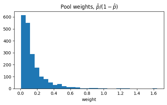
IPTW relies on positivity: every pool patient needs a realistic chance of looking like the target on the fitted model. A propensity score distribution piled up near 0 or 1, or a handful of huge weights, is the practical warning sign – the reweighting is leaning hard on a small, possibly unrepresentative slice of the pool (the same concern effective_sample_size() summarizes in one number).

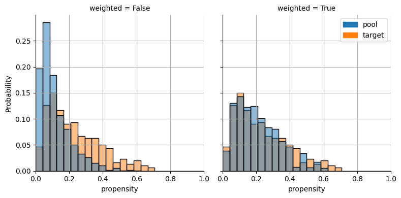
plot_iptw_propensity_distributions() is the weighting counterpart to pybalance.propensity.plot_propensity_score_match_distributions(): instead of a matched subset’s “before” vs. “after” panels, it shows the same pool/target propensity scores counted equally (“before”) vs. counted by the fitted IPTW weight (“after”) – the weighted pool histogram should move towards the target’s.

plot_iptw_propensity_distributions(weighter);

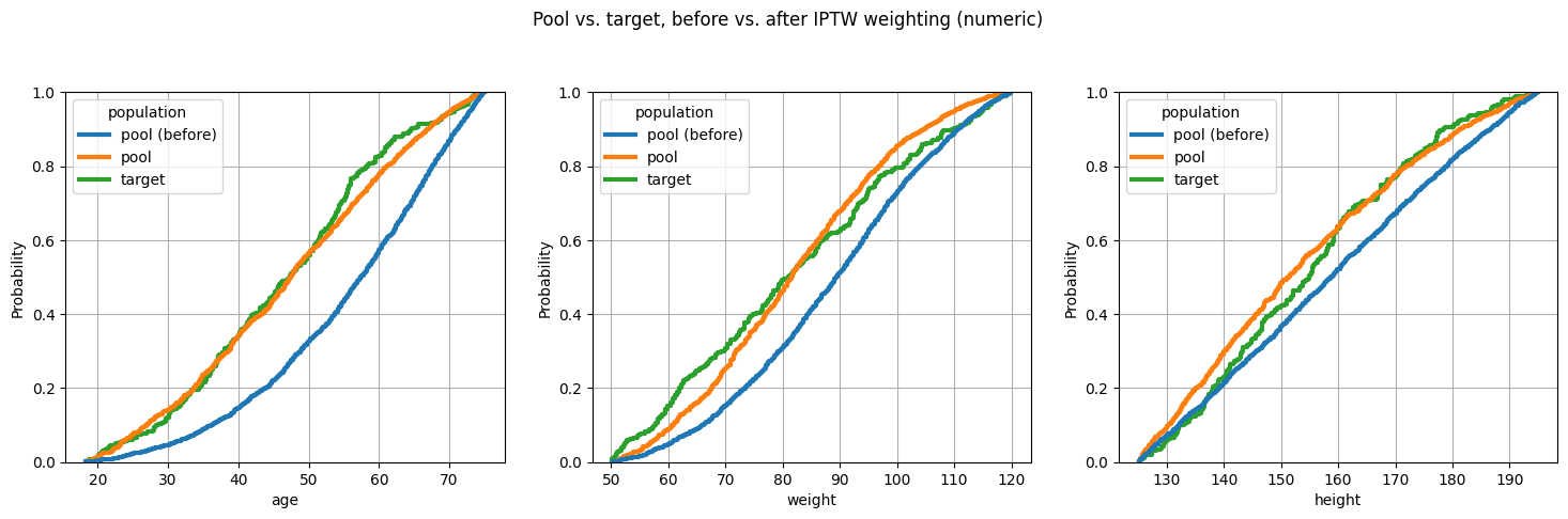
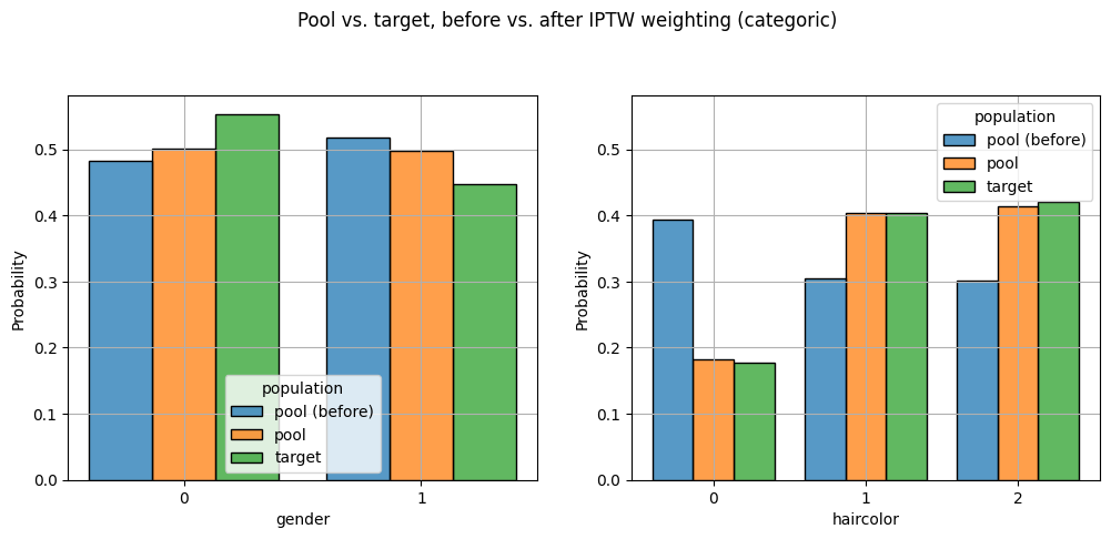
Both plot_numeric_features and plot_categoric_features accept a weights= column, so the unweighted pool (every patient counted equally) and the IPTW-weighted pool can be plotted side by side against the same target, to see what the reweighting actually bought.

fig, ax = plt.subplots(figsize=(5.5, 3.5))
ax.hist(weighter.weights, bins=30)
ax.set_title(r"Pool weights, $\hat{p} / (1 - \hat{p})$")
ax.set_xlabel("weight")
fig.tight_layout()

To see the effect on the covariates themselves (rather than the propensity score), put the unweighted pool, the IPTW-weighted pool and the target into a single MatchingData – the same trick the matching demos use to show “pool (prematch)” alongside “pool” and “target” in one plot – and pass weights= through to plot_numeric_features/plot_categoric_features. The unweighted pool copy gets weight 1, so a single call draws all three distributions together instead of two separate before/after figures.

before_pool = matching_data.get_population(matching_data.pool_name).copy()
before_pool[weighter.weight_col] = 1.0

combined = matched.copy()
combined.append(before_pool, name="pool (before)")
hue_order = ["pool (before)", matching_data.pool_name, matching_data.target_name]

plot_numeric_features(
    combined, weights=weighter.weight_col, hue_order=hue_order, include_only=headers.numeric, col_wrap=3
)
plt.suptitle("Pool vs. target, before vs. after IPTW weighting (numeric)", y=1.05);

plot_categoric_features(
    combined, weights=weighter.weight_col, hue_order=hue_order, include_only=headers.categoric, col_wrap=2
)
plt.suptitle("Pool vs. target, before vs. after IPTW weighting (categoric)", y=1.05);

Trimming extreme weights

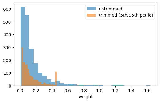
The main practical failure mode of IPTW is a small number of extreme weights, driven by pool patients whose covariates make the model almost certain they’re pool (weight -> 0) or almost certain they’re target (weight -> large). trim_quantiles=(low, high) clips fitted weights at the given quantiles – a standard bias/variance trade-off: a little exact balance is sacrificed in exchange for a much more stable, lower-variance set of weights.

trimmed = IPTWWeighter(matching_data, trim_quantiles=(0.05, 0.95), verbose=True)
trimmed.match()

print(f"Untrimmed: ESS={weighter.effective_sample_size():.1f}, max weight={weighter.weights.max():.2f}")
print(f"Trimmed:   ESS={trimmed.effective_sample_size():.1f}, max weight={trimmed.weights.max():.2f}, n_trimmed={trimmed.diagnostics['n_trimmed']}")

fig, ax = plt.subplots(figsize=(6, 3.5))
ax.hist(weighter.weights, bins=30, alpha=0.6, label="untrimmed")
ax.hist(trimmed.weights, bins=30, alpha=0.6, label="trimmed (5th/95th pctile)")
ax.set_xlabel("weight")
ax.legend();

IPTWWeighter fit LogisticRegression. Effective sample size: 1148.0 / 2000 pool patients. Trimmed 200 extreme weights.

Untrimmed: ESS=946.5, max weight=1.64
Trimmed:   ESS=1148.0, max weight=0.46, n_trimmed=200

Takeaways

• IPTWWeighter fits a pool-vs-target propensity model and weights the pool by \(\hat p / (1 - \hat p)\); the target keeps weight 1 (the ATT estimand, target-as-reference).

• It requires a patient-level target – there’s no aggregate-only (“published Table 1”) variant.

• It does not solve for exact balance, so always check weighted_balance_table() and effective_sample_size() on the fitted result, the same as for any other weighter.

• trim_quantiles caps extreme weights, trading a little bias for a large reduction in variance – worth reaching for whenever a handful of patients end up dominating the effective sample size.