MARTINI - MLAI pipeline prepare module • martini

Scope

Package

The MARTINIprep package is the first part of the BMDI MARTINI pipeline, which aims at assessing the relation of baseline information from clinical domains with a given outcome. MARTINIprep provides a convenient framework to gather information from different clinical data sets and to combine them into a machine-learning-ready data set. The output is meant to be used with packages MARTINImodtune and MARTINIreport, both included in the MARTINI meta package (to come).

The automated part of the preparation workflow is handled by the three main functions of MARTINIprep, namely

adam_spec(),
ads_build(),
prepare_ml().

The package was developed in the clinical context which is reflected in the default settings and specifics of both the main and helper functions. This vignette is solely focused on the standard clinical setting. However, the functions may also be used with more general data sets, please refer to the individual help pages for full details.

Vignette

This vignette serves as a hands-on tutorial on the usage of the MARTINIprep package. It clearly outlines the required steps to get from an ads folder to a machine learning data set, listing a number of commonly required adaptations along the way.

The package comes with a number of example data sets, ranging from raw sas data sets to be read in, to data objects representing intermediate steps (e.g. martini_spec, martini_feat) as well as the final output object (martini_ml_class) for further use in the

modules of the pipeline.

High-level concept

In the (admittedly unrealistic) case that no manual adaptations have to be made to the data contained in the ADaM data sets included in the analysis, the full preparation could be accomplished by running the composed command

path %>% 
  adam_spec() %>% 
  build() %>% 
  prepare_ml(outcome = outcome_data)

where path would be defined as the location where the ADaM data sets are stored in .sas7bdat format. The chart below highlights the main workflow and lists related helper functions (mostly internal).

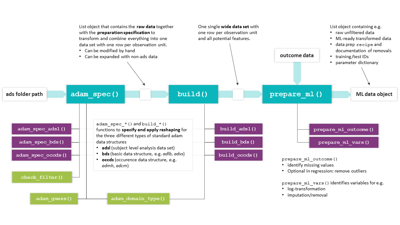
Overview of MARTINIprep functions. The basic workflow from ads path to ML data object is accomplished by the main functions (turquoise), which make use of the (mostly internal) helper functions shown below.

Outcome preparation

It is recommended to clearly define the outcome of interest and prepare the outcome data set independently from the feature engineering process. The outcome data set may contain information on different endpoints in a single tibble, with one row per id and the different outcomes in the columns. In practice, separate data sets for each outcome are preferable for large studies, considering the potentially higher preparation times. For time-to-event data, each endpoint is described by two columns (representing time and status, resp.).

Since the analysis of survival endpoints is computationally much more expensive than for classification, the latter may be used for initial runs by using a dichotomized version of the endpoint (i.e. event yes/no in given time frame). When binarizing time-to-event endpoints, please pay attention to the study duration (potentially reduce to subjects with minimum time under observation) and the resulting outcome distribution (highly unbalanced data, low event rate?).

The package comes with two exemplary outcome data sets, one for classification, one for a regression problem. Both are two column tibbles with an .id and an .out column, where in the classification example shown below, the .out variable is a factor with two levels (event/no event).

For survival, the outcome information would be coded in two separate columns, e.g. days and event. Note that for the specification of the outcome names for prepare_ml(), a named vector is expected in the survival case, e.g. outcome_names = c(.time = 'days', .status = 'event').

martini_outc_class %>% 
  head(3) %>% 
  kableExtra::kable() %>% 
  kableExtra::kable_styling(full_width = FALSE)

Please note that currently, only binary classification is fully supported by the MARTINI pipeline.

Time-to-event preparation

For convenience, the package also provides build_out_tte(), which allows to prepare a tte-based outcome for further use with prepare_ml(). Starting from either file (specifying the path to an ADaM adtte.sas7bdat) or an already existing data object with the same structure, the user has the option to prepare either a tte outcome or a binarized version. In the latter case, a duration of interest has to be specified in cut and the resulting endpoint translates to e.g. event in first 2 years (yes/no). Make sure, that the scale of cut matches the scale of the time column, i.e. if AVAL is in days, cut has to be in days, no conversion is done internally. cut is provided as numeric, not object of class duration.

build_out_tte(
  
  # either file or data have to be provided
  file    = 'adtte.sas7bdat',
  
  # select e.g. parameter of interest, subset to population
  filter  = 'PARAMCD == "CVDEATH"', 
  
  # AVAL is in days, cut is used as threshold 
  cut     = 365*2
)

Please note, that while the full population will be used for tte outcomes, the population for the binarized version is subsetted: Patients are discarded, if a censored event was recorded with a time below the cutoff of interest (here 2 years). If a patient has not been observed for the duration of cut, there is no information on whether or not an event occurred within cut.

Example study MARTINI

Assume an example study containing four data sets in .sas7bdat format, covering the three different ADaM data types:

adsl (adsl, wide format)
adlb (bds, long format)
advs (bds, long format)
admh (occds, long format)

These data sets will be used to illustrate how to make manual adaptations in order to customize the preparation process to a particular analysis and research task.

In addition to these raw data sets, the following data sets are available as examples for the intermediate data sets produced during the preparation process:

martini_spec result of adam_spec() applied to ads folder
martini_feat result of build(), a wide data set containing information of all selected domains
martini_outc_regr, martini_outc_class prepared outcome data sets (in practice, e.g. from adtte)
martini_ml_regr, martini_ml_class result of prepare_ml(), to be used in MARTINImodtune and/or MARTINIreport

We will focus on the description of the main functions, but each package function (exported or not) has its own help page, so feel free to learn more about the detailed functionality on the individual pages.

Getting started

In the setting of clinical studies, we assume that a set of analysis data sets (ads) is stored in .sas7bdat format in a single folder path.

After specifying the folder location

# path <- 'path/to/sasfiles'
path <- system.file(
  "martini_example_study", "ads", 
  package = "martini", mustWork = TRUE
)

you may check beforehand which data sets can be processed automatically to make sure, all information of interest can be incorporated in the analysis. Running

adam_domain_type(path)

returns a tibble with the name of the domain, its mapped ADaM data types (occds/adsl/bds) along with the full file path. For domains with type=='none' no mapping information is available (yet) and the data set would not be processed automatically.

In case a particular domain is required for your analysis but not included in the current list, please get in touch with the package maintainers (Sebastian Voss, Maike Ahrens).

adam_domain_type(path)
#> # A tibble: 4 × 4
#>   domain type  file_ext file                                                    
#>   <chr>  <chr> <chr>    <chr>                                                   
#> 1 adlb   bds   sas7bdat /home/runner/work/_temp/Library/martini/martini_example…
#> 2 admh   occds sas7bdat /home/runner/work/_temp/Library/martini/martini_example…
#> 3 adsl   adsl  sas7bdat /home/runner/work/_temp/Library/martini/martini_example…
#> 4 advs   bds   sas7bdat /home/runner/work/_temp/Library/martini/martini_example…

TL;DR


d_ml <- path %>% 
  
  # create automated spec
  adam_spec() %>% 
  
  # make adjustments
  adjust_adsl("adsl", drop = c("AGEGR01")) %>% 
  adjust_spec("admh", count = FALSE) %>% 
  
  # build combined wide data set
  build() %>% 
  
  # prepare data for ml
  prepare_ml(outcome = martini_outc_class)

Pay attention to the output in the console. If applicable, the following information will be provided

adam_spec()
- data sets that could not be processed automatically
- assessment of the filter applicability
build()
- bds-type data sets with duplicate measures will be reported. Duplicates may be indicative of missing filters (e.g. ABLFL == 1), thus resulting in incorrect data preparation. Check back with the information on filters applied to the respective data set.

`adam_spec()`

The adam_spec() function creates a preprocessing specification in the form of a list from a given path. Each entry contains the required information to extract relevant records from a particular data set and reshape the data into wide format. The structure of the top level entries depends on the type of the corresponding data set (adsl/bds/occds).

Among other steps, adam_spec() will

generate md5 checksums
identify data sets that can be processed automatically (by matching file names against an internal library)
check applicability of provided filters
create a parameter dictionary

In general, this automatically created specification may be used with the subsequent workflow, however, in practice, it will be modified by the user to match specific requirements.

Printing the spec object to the console will provide information on data set size, derived numbers of columns and subjects (after filter application).

ads_spec <- adam_spec(path)
ads_spec
#> 
#>   Content
#>   name type   size nsubj ncol
#>   adsl adsl   128K   320    7
#>   adlb bds   1.31M   289   11
#>   advs bds    448K   289    5
#>   admh occds  192K   320    2
#> 
#>   Key columns used in bds-type data sets
#>   name param   value unit  time  
#>   adlb PARAMCD AVAL  AVALU AVISIT
#>   advs PARAMCD AVAL  AVALU AVISIT
#> 
#>   Key columns used in occds-type data sets
#>   name label  value valuen count time  
#>   admh MHHLGT NA    NA     TRUE  MHSTDY

Make yourself familiar with the list structure and contained information of the spec object:

ads_spec %>% str(max.level = 1)
#> List of 4
#>  $ adsl:List of 16
#>   ..- attr(*, "filter_ok")= logi TRUE
#>   ..- attr(*, "data_info_ok")= logi TRUE
#>  $ adlb:List of 17
#>   ..- attr(*, "filter_ok")= logi TRUE
#>   ..- attr(*, "data_info_ok")= logi TRUE
#>  $ advs:List of 17
#>   ..- attr(*, "filter_ok")= logi TRUE
#>   ..- attr(*, "data_info_ok")= logi TRUE
#>  $ admh:List of 16
#>   ..- attr(*, "filter_ok")= logi TRUE
#>   ..- attr(*, "data_info_ok")= logi TRUE
#>  - attr(*, "class")= chr [1:2] "martini_spec" "list"

adsl column selection

In contrast to occds and bds type data, an automated column selection is required for the wide format adsl data sets.

Reasons for column exclusion are documented in the drop_list entry of the corresponding spec entry. Exclusion criteria include, but are not limited to datetime/duration-related columns or analysis set flags.

ads_spec$adsl$drop_list %>% names()

Important parameters

Filters

The filter argument takes a character vector of expressions to be passed to dplyr::filter(). A filter will be applied to a particular data set only if its (individual) application yields a non-empty tibble (i.e. no error thrown, at least one row is selected). In addition, the function will throw a message, if the combination of all valid filters would yield an empty data set.

Common filters may be based on visit or treatment information, as well as flags indicating analysis sets. If a filter should be applied to only one particular ads domain and not considered for the other domains, just add the respective ADSNAME column (for standard data sets), e.g. "ADSNAME == 'ADVS' & AVISIT == 'Visit 1'".

The pre_study argument allows to conveniently reduce occurrence data sets (e.g. medical history records) to data that is available at baseline based on the study day.

Filters have to be adjusted for the data at hand, find below a list of exemplary filters:

filters  <- c(
  
  # use only baseline data
  "AVISIT == 'Baseline'",
  "ABLFL == 'Y'",
  
  # no baseline visit in advs domain, use visit 1 instead
  "AVISIT == 'Visit 1' & ADSNAME == 'ADVS'",
  
  # ITT population
  "ITTFL == 'Y'",
  "!is.na(TRT01A)",
  
  # exclude a single parameter 
  "PARAMCD != 'BPDIA'",
  
  # some MH and CM entries have a Y/N coding (but not all)
  "MHOCCUR == 'Y' | is.na(MHOCCUR)",
  "CMOCCUR == 'Y' | is.na(CMOCCUR)"

)

ads_spec <- adam_spec(
  path, 
  filter    = filters, 
  pre_study = TRUE
)

An overview of applied and discarded filters from the filters provided to \link{adam_spec}() is printed to the console when calling \link{adam_spec}() as well as when printing the object to the console. The filter set that was originally provided to \link{adam_spec}() is stored in the filter attribute of the resulting object. Note that the print will only refer to this initial filter set and ignore any manual adjustments. We strongly advise to not change filters using spec adjustments but only by rerunning \link{adam_spec}() to assure proper checks.

Always double check the filters that were not applied, typically it is due to

typos
misspecified filter expressions (e.g. = instead of ==)
targeted domain no longer included in the analysis

ads_spec

add_bds

adam_spec() will print a list of domains that are not processed automatically, which are the ones that are not included in the internal package library of domains and corresponding data types.

You may use the add_bds argument of adam_spec() to force them being treated as bds data sets. For these added data sets, it is particularly important to check the automated column selection (in the resulting spec object) and adjust as needed using adjust_spec().

ads_spec <- adam_spec(
  path,
  add_bds = 'adfapr'
)

# print to check the key column definition
ads_spec

Domain selection

Use keep/drop arguments in adam_spec() to select/deselect particular data sets in the folder path for your analysis. Only selected files will be read in order to create a specification, so these parameters directly impact run time.

An example for a reasonable exclusion of a data set would be e.g. a data set on biomarkers that were measured only for a small subpopulation (by default, data sets are combined using inner_join(), but it’s a parameter to build()).

Attach data

In order to create a data set specification, the data set has to be read first which may take a considerable amount of time for large files. For a more time-efficient usage, the data sets may be stored directly in the ads_spec object from where the actual execution of the preparation will be conducted.

In the current implementation, if changes to any of the data sets shall be made (see below), all data sets have to be attached.

ads_spec <- adam_spec(
  path, 
  attach_data = TRUE
)

Using rds data

For martini version >=0.5.1, not only files but also data in rds format may be used (see argument in ).

If for instance, only particular treatment groups or visits are considered for an analysis , filtering the original data sets and storing them as , may speed up the data preparation significantly for larger data sets.

Suppose all domains of interest are available in a subset/filtered version and stored as data in .

ads_spec <- adam_spec(
  path, 
  file_ext = 'rds'
)

Manual adaptations

After the initial spec was created, the user should inspect the object and make necessary adjustments. It is strongly recommended to use the build-in helper functions where possible, since they provide some basic checks of the desired modifications in terms of consistency and applicability.

Variable selection from adsl

A common task is to review and adjust the automated variable selection from adsl by inspecting martini_spec$adsl$dict (or simply martini_spec$adsl$select).

Reasons for dropping variables from the automated selection may include but are not limited to:

post baseline information (MARTINI pipeline aims at assessing the relation of baseline information with a given outcome. Consequently, outcome-related information should be removed (e.g. death flag))
variables are available in both a continuous as well as categorical version (e.g. age, BMI, weight), there is no automated selection available
different groupings based on the same variable (e.g. country group)

The adjustment can be accomplished by using the adjust_adsl_select() function, which allows to either add or drop variables from the automated selection. Small adjustments can be made using the drop and add arguments, but the user can also provide the exact set of variables to extract using the select argument. In the latter case, make sure to include the variables with special roles id and trt in the adam_spec() function to avoid the corresponding warnings.

martini_spec <- martini_spec %>% 
  adjust_adsl_select(
    add  = c('BMI'),
    drop = c('AGE')
  )

martini_spec <- martini_spec %>% 
  adjust_adsl_select(
    select = c("SUBJID", "TRT01A", "SEX", "RACE", "AGE", "BMI")
  )

# warnings for missing id and trt
martini_spec <- martini_spec %>% 
  adjust_adsl_select(
    select = c("SEX", "RACE", "AGE", "BMI")
  )

For large data sets, the creation of the select vector may be cumbersome. In this case, it may be helpful to extract the current selection and adjust it using e.g. the stringr::str_subset() function to make use of regular expressions.

user_selection <- ads_spec$adsl$select %>% 
  
  # remove post baseline information
  setdiff(c('DEATHFL')) %>% 
 
  # categoricals with a continuous version 
  str_subset("AGEGR|BMIGR|WEIGGR|RACEGR", negate = TRUE) %>% 

  # several grouped versions available
  str_subset("CNTYGR[2-7]")

The removal of variables that are not derived from adsl, but from one of the long format data sets, the removal is actual accomplished by applying a filter, please refer to the section on adjust_filter() for more information.

Factor levels in adsl

The function adjust_adsl_factors() can be used to adjust or expand the factor level list. The level order will determine for example the display order in tabular outputs in certain contexts.

In the following example, the factor level order for the variable RACE is reversed and labels are changed to lower case. Assigning factor labels is particularly useful for variables that were automatically identified as factors, but do not have the desired labels (e.g. due to missing decode column as typical for ADaM 2.0 and/or issues with reading the label information from the sas catalog file).

martini_spec <- martini_spec %>% 
  adjust_adsl_factors(
      fctrs = list(
        "RACE" = c(asian = "ASIAN", black = "BLACK", white = "WHITE")
      )
  )

In addition to reordering and relabeling existing factors in the list, it is also possible to add variables to the factor list that would have been dropped otherwise.

Note, that the factor level list contains information on all detected factors, irrespective of whether they are selected or not. Refer to adsl’s dictionary (selected) to see which factor levels are actually applied.

martini_spec <- martini_spec %>% 
  adjust_adsl_select(add = "AGEGR01N") %>%
  adjust_adsl_factors(
      fctrs = list(
        "AGEGR01N" = c("< 60" = 1, "60 - <75" = 2, ">=75" = 3)
      )
  )

Filters

The function adjust_filter() allows to update the set of filters for the martini_spec object. If an error in the filter expression is detected during the inspection of the spec object, e.g. in the filter information section of the console output from printing, the set of filters can be adjusted easily without rerunning the adam_spec() as long as the data is attached. If no data is attached, the filter checks cannot be performed and adam_spec() should be re-run to avoid any downstream issues.

General adjustments

The adjust_spec() function allows to adjust the parameter of a particular entry of the spec object, related to the data extraction, such as param and label for bds entries or value and count for occds entries.

Some entries are protected from manual adjustments altogether, adjustments of entries filter, factor_levels and column selection from adsl the respective specialized functions should be used (adjust_filter(), adjust_adsl_select(), adjust_adsl_factors()).

Value column for bds type data

In order to create a wide data set from bds type data, the main operation is the application of tidyr::pivot_wider(). adam_spec will guess the appropriate columns to use for names_from and values_from (if not provided) and store them in the list entries param and value of the respective spec entry, respectively, e.g. param = PARAMCD and value = AVAL.

Please do check the entries before moving on to build() to ensure correct handling of variable types. If necessary, use adjust_spec() to make any changes.

For some domains, variables may differ in type, i.e. while some are numeric (and AVAL) should be used, others might be available in character format (e.g. high/low, where AVALC). Appropriate handling depends on the exact data structure:

If AVALC also contains the numeric values, build() is able to handle variables differently based on their (guessed) type, i.e. convert character values from AVALC to either factors or numerics based on observed values.
If AVALC and AVAL contain complementary information (AVALC missing values for numeric variables):
- create new (character) column combining AVALC and AVAL and adjust attached data and spec entry value accordingly
- create two disjoint spec entries for the same data set: filtering for numeric and character variables, respectively, by setting filters manually (e.g. based on PARAMCD) and choosing the appropriate value column for each subset

Add data

In order to add new (external) data, simply add a new entry in the existing ads_spec object. Depending on the type of data to add, create a list that has the same structure as the relevant exemplary one above.

ads_spec$add <- list(
  file = file_to_add,
  md5  = tools::md5sum(file),
  data = additional_data,
  type = 'adsl',
  ...
)

This approach is preferable to adding data e.g. to the data slot of adsl since it makes sure that the extracted variables will appear in the data dictionary with the appropriate data source (name of spec entry).

Change data set label

adam_spec() automatically selects a label column in occds data sets (e.g. admh), that controls the categorization of the occurrences and defines the variables that are created by the build() function. If you need a more or less detailed categorization, you need to change the label entry.

# change label column in admh
ads_spec %>% 
  adjust_spec(
    id = 'admh',
    label = "MHBODSYS"
  )

# equivalent to
# ads_spec $admh$label <- "MHBODSYS"

Handling of occurrence data

When trying to extract information from an occurrence data set (such as admh, adcm, adxa) in a binary manner (e.g. particular medication yes/no), a lot of the resulting variables may be discarded in the data preparation process due to near-zero variance.
In order to keep at least some information, the default for occds data set preparation is to simply count the number of entries, as commonly a higher number of entries roughly translates to a worse status.

If the count option is used, check that none of the entries is equivalent to no record (e.g. value ‘none’ in adjuvant therapy). These values should be excluded using the filter parameter in the adam_spec() function beforehand.

If instead individual variables should be derived, the user may set the count value in the corresponding spec to ‘FALSE’.

ads_spec$admh$count <- FALSE

If one does not opt for the count option, but for individual variables, there is also the possibility to specify a valuen column, which in the case of adae may be set to the column indicating the severity of the event. Analogously, a value entry may be provided for non-numeric information, e.g.

ads_spec %>% 
  adjust_spec('admh', value = 'MHPRESP')

# equivalent to
# ads_spec$admh$value <- 'MHPRESP'

`build()`

Based on a given ads_spec object (modified or generated fully automatically), the build() function will execute the extraction of the relevant information according to the ads_spec entries and combine everything into a single (wide) data set. This data set is the basis for the feature matrix used later on for machine learning.

By default, the resulting (wide) data set will have one row per id. For the analysis of repeated measurement outcomes, one row needs to correspond to one subject at a given timepoint, which can be achieved by setting rm = TRUE.

feature <- build(
  spec,
  rm = FALSE  
)

Adding or modifying wide data set after build()

The output object of build() is a wide data set, with a dictionary attribute containing information on the variables and their origin. If the data set is to be used with the martini pipeline it is crucial that the dictionary is consistent with the provided data set.

recoding of factors (e.g. summarising levels)
deriving new variables (e.g. clinical index or summary scores from questionnaires or interaction terms)


feature <- feature %>% 
  mutate(RACE = fct_collapse(RACE, other = c("asian", "black"))) %>% 
  mutate(RISK_CLASS = case_when(
    BMI >= 30 & CREAT >= 2 ~ "III",
    BMI >= 30 & CREAT <  2 ~ "II",
    TRUE ~ "I"
  ) %>% factor())

#

`prepare_ml()`

Once all potential features are available in a single data set, the prepare_ml() function will take care of the data preprocessing required for machine learning analysis based on the provided outcome data.

ml_data <- prepare_ml(
  feature, 
  outcome
)

Please refer to the help pages of prepare_ml() for information on the required structure of outcome for single vs repeated measurement outcomes.

Data splitting

Splitting the data in training and test data will create a 3:1 split by default, stratified by outcome if appropriate. To include treatment information in the stratification, set strata_trt = TRUE.

Preprocessing

While each step is optional and parametrized to provide maximum flexibility to the user, default parameters were chosen carefully and may be considered appropriate for a large number of analyses.

The preprocessing includes the following steps

splitting in training and test set (stratified by e.g. treatment)
removal of noise
reduction of multicollinearity by removing highly correlated variables
log-transformation of highly skewed variables
normalization
imputation
dummy coding

NOTE: Please be aware that in the initial versions, dummy coding was set to TRUE by default. From version 0.2 on, the default is FALSE which is appropriate for most applications.

Inspect d_ml objects

data("martini_ml_class")
d_ml <- martini_ml_class
str(d_ml, max.level = 2)
#> List of 10
#>  $ data_raw   :List of 2
#>   ..$ train: tibble [215 × 27] (S3: tbl_df/tbl/data.frame)
#>   ..$ test : tibble [74 × 27] (S3: tbl_df/tbl/data.frame)
#>  $ data_prep  :List of 2
#>   ..$ train: tibble [215 × 25] (S3: tbl_df/tbl/data.frame)
#>   ..$ test : tibble [74 × 25] (S3: tbl_df/tbl/data.frame)
#>  $ outcome    :List of 2
#>   ..$ name: chr ".out"
#>   ..$ mode: chr "classification"
#>  $ dict       : tibble [27 × 10] (S3: tbl_df/tbl/data.frame)
#>  $ source     : tibble [4 × 3] (S3: tbl_df/tbl/data.frame)
#>  $ prep_recipe:List of 11
#>   ..$ var_info      : tibble [27 × 4] (S3: tbl_df/tbl/data.frame)
#>   ..$ term_info     : tibble [25 × 4] (S3: tbl_df/tbl/data.frame)
#>   ..$ steps         :List of 15
#>   ..$ template      : tibble [215 × 25] (S3: tbl_df/tbl/data.frame)
#>   ..$ retained      : logi TRUE
#>   ..$ requirements  :List of 1
#>   ..$ ptype         : tibble [0 × 27] (S3: tbl_df/tbl/data.frame)
#>   ..$ tr_info       :'data.frame':   1 obs. of  2 variables:
#>   ..$ orig_lvls     :List of 27
#>   ..$ fit_times     : tibble [30 × 2] (S3: tbl_df/tbl/data.frame)
#>   ..$ last_term_info: gropd_df [27 × 6] (S3: grouped_df/tbl_df/tbl/data.frame)
#>   .. ..- attr(*, "groups")= tibble [27 × 2] (S3: tbl_df/tbl/data.frame)
#>   .. .. ..- attr(*, ".drop")= logi TRUE
#>   ..- attr(*, "class")= chr "recipe"
#>  $ prep_params:List of 7
#>   ..$ thres_log     :List of 2
#>   ..$ thres_count   :List of 2
#>   ..$ thres_corr    :List of 2
#>   ..$ vars_keep_corr:List of 2
#>   ..$ thres_lump    :List of 2
#>   ..$ imp_ignore    :List of 2
#>   ..$ nzv           :List of 2
#>  $ removed    :List of 2
#>   ..$ rows:List of 3
#>   ..$ cols:List of 4
#>  $ high_corr  : tibble [2 × 3] (S3: tbl_df/tbl/data.frame)
#>  $ input      :List of 2
#>   ..$ martini:Classes 'package_version', 'numeric_version'  hidden list of 1
#>   ..$ args   :List of 25

Description of the d_ml entries (taken from martini::prepare_ml() documentation)

Data sets

prepare_ml() produces a list that contains the data set both with (data_prep) and without (data_raw) applying the specified ML preparation steps. Both versions are split in train and test set. In addition, split contains the combined rsample::initial_split() object that the train and test data was extracted from. Depending on the programming workflow, one might be more convenient to use than the other.

For convenient extraction of the full, i.e. unsplit, data set, one may use `get_data():

# by default, prepared data is extracted
prep <- get_data(d_ml)

# get raw version of data
raw  <- get_data(d_ml, type = 'raw')

# keep information on which set the observation was in (train/test)
raw  <- get_data(d_ml, type = 'raw', split_id = 'train_test')

either raw or prepared data

The slot outcome contains a list giving name, the standardized names of the output column in the data sets (.out for regression/classification, .time and .status for survival), as well as mode, a character string of the outcome mode regression/classification/survival.

The dictionary available as an attribute of feature is updated with information on the outcome variable and the log-transformation and available from the dict slot, NULL if no such attribute is defined. Columns label2 and label3 provide additional information on correlation structure in the data set: (variables removed for correlation).

The source slot simply passes the source attribute of feature, NULL if no such attribute is defined. If build() from the martini package was used to generate feature, this attribute lists the full paths of the files that were used in data generation of feature.

Avoiding downstream issues

In some applications, issues were observed if the training data set contains factors with low frequency classes. These may cause issues in the tuning process, most likely in the cross-validation steps. Please note, that this is in fact an issue with the implementation of ranger, which is currently being worked on. Since there is no generally best solution on the data prep side, we provide a helper function that may at least help in the identification of the variables causing the issue:

check_freq() will check the prepped training data of a given ml object (result of prepare_ml()) for factors that may cause problems in this regard.

d_ml %>%  
  check_freq(thres = 25)

In case factors with low frequency classes are identified, the corresponding frequency tables are returned in a list.

Data preparation and documentation

prep_recipe contains the prepared recipe object, prep_params documents the parameters/thresholds used in the data preparation, giving bare value slots, as well as a verbose description in text. removed gives a list of removed rows and columns along with the information on why/in which recipe step the data was removed.
If data_prep has less columns than data_raw, details on removal can be found in d_ml$removed$cols.

d_ml$removed$cols %>% 
  enframe() %>%  
  unnest_longer(value) %>% 
  left_join(
    d_ml$dict %>% select(value = column, source, label),
    ) %>% 
  rename(reason = name, `variable removed` = value)
#> Joining with `by = join_by(value)`
#> # A tibble: 2 × 4
#>   reason `variable removed` source label                     
#>   <chr>  <chr>              <chr>  <chr>                     
#> 1 nzv    angina_pectoris    admh   Angina pectoris           
#> 2 corr   HB                 adlb   Hemoglobin (g/dL) in Blood

If data_prep has less rows than data_raw, details on removal can be found in d_ml$removed$rows. Observations are removed if
- no outcome is available
- outcome value was identified as outlier (regression only, optional, parametrized)
- the value for a variable is missing, that is excluded from imputation (e.g. trt), but the missing value proportion is considered low enough that the observations are dropped (instead of dropping the variable)

d_ml$removed$rows
#> $outlier_outcome
#> NULL
#> 
#> $na_outcome
#> NULL
#> 
#> $na_feature
#> NULL

d_ml$data_raw %>% 
  bind_rows() %>% 
  filter(.id %in% d_ml$removed$rows$na_feature)

For validation and transparency, all domains used for feature extraction are listed with full paths and md5 check sums.

d_ml$source

Group specific modelling (e.g. treatment versus placebo)

In order to assess treatment interactions, a group specific modelling approach has been established for the MARTINI pipeline (#melon app). For the comparability of results across groups, it is crucial that the data preparation is identical (e.g. in terms of coefficients for the normalization).

Given an output object of prepare_ml() and a character defining the name of the by variable (factor) to split by, prepare_ml_split() will return separate ml data sets for each factor level to be used with the remainder of the MARTINI modules. Note that the by variable is constant in each subset, thus removed from the feature set in the prepared data, but still available in the raw data sets.

MARTINI - MLAI pipeline prepare module

A hands-on tutorial on the preparation of ADaM data for Machine Learning

Maike Ahrens, Sebastian Voss