Matching Data
In this notebook, we demonstrate the MatchingData class, which organizes population data for matching, and some plotting tools for visualizing the data. You can download this notebook to run yourself here: https://github.com/Bayer-Group/pybalance/blob/main/sphinx/demos/matching_data.ipynb.
[1]:
import os
import logging
logging.basicConfig(
    format="%(levelname)-4s [%(filename)s:%(lineno)d] %(message)s",
    level='INFO',
)

import pandas as pd

import pybalance
from pybalance import MatchingData, MatchingHeaders, split_target_pool
from pybalance.visualization import (
    plot_numeric_features,
    plot_categoric_features,
    plot_binary_features,
    plot_joint_numeric_distributions,
    plot_joint_numeric_categoric_distributions,
    plot_per_feature_loss
)
from pybalance.sim import get_paper_dataset_path
Initializing MatchingData
The MatchingData class is a thin wrapper around pandas DataFrame that additionally keeps track of certain metadata about the columns relevant for matching. MatchingData can be initialized from either a string or pandas DataFrame.
[2]:
# initialize MatchingData from path
data_path = get_paper_dataset_path()
m = MatchingData(data=data_path)
m
[2]:
['age', 'height', 'weight']
Headers Categoric:
['gender', 'haircolor', 'country', 'binary_0', 'binary_1', 'binary_2', 'binary_3']
Populations
['pool', 'target']
| age | height | weight | gender | haircolor | country | population | binary_0 | binary_1 | binary_2 | binary_3 | patient_id | |
|---|---|---|---|---|---|---|---|---|---|---|---|---|
| 0 | 64.854093 | 189.466850 | 88.835049 | 1.0 | 1 | 4 | pool | 0 | 1 | 0 | 1 | 135740 |
| 1 | 52.571993 | 158.134940 | 94.215107 | 1.0 | 1 | 1 | pool | 0 | 1 | 0 | 1 | 49288 |
| 2 | 25.828361 | 154.692482 | 94.226222 | 1.0 | 0 | 3 | pool | 0 | 0 | 1 | 0 | 256676 |
| 3 | 70.177571 | 160.536632 | 94.244356 | 1.0 | 0 | 2 | pool | 0 | 0 | 0 | 1 | 338287 |
| 4 | 73.779164 | 153.551419 | 86.161814 | 0.0 | 0 | 1 | pool | 0 | 0 | 1 | 1 | 72849 |
| ... | ... | ... | ... | ... | ... | ... | ... | ... | ... | ... | ... | ... |
| 274995 | 62.547794 | 186.005015 | 50.975051 | 0.0 | 0 | 1 | target | 0 | 0 | 1 | 1 | 579081 |
| 274996 | 69.879934 | 142.371386 | 100.138389 | 1.0 | 1 | 4 | target | 0 | 1 | 1 | 0 | 569939 |
| 274997 | 56.921402 | 130.639589 | 108.745182 | 1.0 | 1 | 5 | target | 0 | 1 | 0 | 0 | 532419 |
| 274998 | 34.082754 | 174.764051 | 67.998396 | 0.0 | 2 | 2 | target | 0 | 0 | 0 | 1 | 566266 |
| 274999 | 60.981259 | 137.419436 | 89.897817 | 1.0 | 0 | 5 | target | 1 | 1 | 1 | 1 | 544231 |
275000 rows × 12 columns
[3]:
# initialize MatchingData from pandas DataFrame
data = pd.read_parquet(data_path)
m = MatchingData(data=data)
m
[3]:
['age', 'height', 'weight']
Headers Categoric:
['gender', 'haircolor', 'country', 'binary_0', 'binary_1', 'binary_2', 'binary_3']
Populations
['pool', 'target']
| age | height | weight | gender | haircolor | country | population | binary_0 | binary_1 | binary_2 | binary_3 | patient_id | |
|---|---|---|---|---|---|---|---|---|---|---|---|---|
| 0 | 64.854093 | 189.466850 | 88.835049 | 1.0 | 1 | 4 | pool | 0 | 1 | 0 | 1 | 135740 |
| 1 | 52.571993 | 158.134940 | 94.215107 | 1.0 | 1 | 1 | pool | 0 | 1 | 0 | 1 | 49288 |
| 2 | 25.828361 | 154.692482 | 94.226222 | 1.0 | 0 | 3 | pool | 0 | 0 | 1 | 0 | 256676 |
| 3 | 70.177571 | 160.536632 | 94.244356 | 1.0 | 0 | 2 | pool | 0 | 0 | 0 | 1 | 338287 |
| 4 | 73.779164 | 153.551419 | 86.161814 | 0.0 | 0 | 1 | pool | 0 | 0 | 1 | 1 | 72849 |
| ... | ... | ... | ... | ... | ... | ... | ... | ... | ... | ... | ... | ... |
| 274995 | 62.547794 | 186.005015 | 50.975051 | 0.0 | 0 | 1 | target | 0 | 0 | 1 | 1 | 579081 |
| 274996 | 69.879934 | 142.371386 | 100.138389 | 1.0 | 1 | 4 | target | 0 | 1 | 1 | 0 | 569939 |
| 274997 | 56.921402 | 130.639589 | 108.745182 | 1.0 | 1 | 5 | target | 0 | 1 | 0 | 0 | 532419 |
| 274998 | 34.082754 | 174.764051 | 67.998396 | 0.0 | 2 | 2 | target | 0 | 0 | 0 | 1 | 566266 |
| 274999 | 60.981259 | 137.419436 | 89.897817 | 1.0 | 0 | 5 | target | 1 | 1 | 1 | 1 | 544231 |
275000 rows × 12 columns
MatchingData will infer which covariates to use for matching and the separation of these into numeric and categoric, unless explicitly specified. Here we specify a subset of the covariates to use for matching. Note that the unused columns are still present in the data, but will simply not be used for matching.
[4]:
headers = MatchingHeaders(
    categoric=['country', 'gender', 'binary_0', 'binary_1'],
    numeric=['age', 'weight', 'height']
)
m_restricted_features = MatchingData(
    data=data,
    headers=headers
)
m_restricted_features
[4]:
['age', 'weight', 'height']
Headers Categoric:
['country', 'gender', 'binary_0', 'binary_1']
Populations
['pool', 'target']
| age | height | weight | gender | haircolor | country | population | binary_0 | binary_1 | binary_2 | binary_3 | patient_id | |
|---|---|---|---|---|---|---|---|---|---|---|---|---|
| 0 | 64.854093 | 189.466850 | 88.835049 | 1.0 | 1 | 4 | pool | 0 | 1 | 0 | 1 | 135740 |
| 1 | 52.571993 | 158.134940 | 94.215107 | 1.0 | 1 | 1 | pool | 0 | 1 | 0 | 1 | 49288 |
| 2 | 25.828361 | 154.692482 | 94.226222 | 1.0 | 0 | 3 | pool | 0 | 0 | 1 | 0 | 256676 |
| 3 | 70.177571 | 160.536632 | 94.244356 | 1.0 | 0 | 2 | pool | 0 | 0 | 0 | 1 | 338287 |
| 4 | 73.779164 | 153.551419 | 86.161814 | 0.0 | 0 | 1 | pool | 0 | 0 | 1 | 1 | 72849 |
| ... | ... | ... | ... | ... | ... | ... | ... | ... | ... | ... | ... | ... |
| 274995 | 62.547794 | 186.005015 | 50.975051 | 0.0 | 0 | 1 | target | 0 | 0 | 1 | 1 | 579081 |
| 274996 | 69.879934 | 142.371386 | 100.138389 | 1.0 | 1 | 4 | target | 0 | 1 | 1 | 0 | 569939 |
| 274997 | 56.921402 | 130.639589 | 108.745182 | 1.0 | 1 | 5 | target | 0 | 1 | 0 | 0 | 532419 |
| 274998 | 34.082754 | 174.764051 | 67.998396 | 0.0 | 2 | 2 | target | 0 | 0 | 0 | 1 | 566266 |
| 274999 | 60.981259 | 137.419436 | 89.897817 | 1.0 | 0 | 5 | target | 1 | 1 | 1 | 1 | 544231 |
275000 rows × 12 columns
Exploring MatchingData
The describe*() methods can be used to generate summary tables of the matching covariates.
[5]:
m.describe(normalize=False)
[5]:
| pool | target | ||
|---|---|---|---|
| population size | N | 250000.00 | 25000.00 |
| gender | 0.0 | 120054.00 | 12956.00 |
| 1.0 | 129946.00 | 12044.00 | |
| haircolor | 0.0 | 100096.00 | 4924.00 |
| 1.0 | 75185.00 | 10055.00 | |
| 2 | 74719.00 | 10021.00 | |
| country | 0.0 | 0.00 | 2490.00 |
| 1.0 | 25033.00 | 5045.00 | |
| 2 | 49534.00 | 4981.00 | |
| 3 | 75337.00 | 2474.00 | |
| 4 | 74934.00 | 5010.00 | |
| 5 | 25162.00 | 5000.00 | |
| binary_0 | 0.0 | 225028.00 | 17535.00 |
| 1.0 | 24972.00 | 7465.00 | |
| binary_1 | 0.0 | 175673.00 | 12527.00 |
| 1.0 | 74327.00 | 12473.00 | |
| binary_2 | 0.0 | 125113.00 | 17472.00 |
| 1.0 | 124887.00 | 7528.00 | |
| binary_3 | 0.0 | 49933.00 | 12562.00 |
| 1.0 | 200067.00 | 12438.00 | |
| age | mean | 55.27 | 48.33 |
| std | 13.18 | 14.39 | |
| min | 18.01 | 18.01 | |
| q25 | 46.38 | 37.29 | |
| median | 57.15 | 48.74 | |
| q75 | 66.10 | 59.85 | |
| max | 75.00 | 75.00 | |
| height | mean | 159.13 | 153.68 |
| std | 19.84 | 16.45 | |
| min | 125.00 | 125.00 | |
| q25 | 142.09 | 140.29 | |
| median | 158.74 | 152.75 | |
| q75 | 175.87 | 165.95 | |
| max | 195.00 | 195.00 | |
| weight | mean | 88.30 | 82.25 |
| std | 16.32 | 18.89 | |
| min | 50.00 | 50.00 | |
| q25 | 76.39 | 66.14 | |
| median | 88.85 | 81.69 | |
| q75 | 100.88 | 97.41 | |
| max | 120.00 | 120.00 |
You can access fields on the underlying data similarly to how you would in pandas.
[6]:
m[['population', 'gender']]
[6]:
| population | gender | |
|---|---|---|
| 0 | pool | 1.0 |
| 1 | pool | 1.0 |
| 2 | pool | 1.0 |
| 3 | pool | 1.0 |
| 4 | pool | 0.0 |
| ... | ... | ... |
| 274995 | target | 0.0 |
| 274996 | target | 1.0 |
| 274997 | target | 1.0 |
| 274998 | target | 0.0 |
| 274999 | target | 1.0 |
275000 rows × 2 columns
[7]:
m[m['gender'] == 0]
[7]:
| age | height | weight | gender | haircolor | country | population | binary_0 | binary_1 | binary_2 | binary_3 | patient_id | |
|---|---|---|---|---|---|---|---|---|---|---|---|---|
| 4 | 73.779164 | 153.551419 | 86.161814 | 0.0 | 0 | 1 | pool | 0 | 0 | 1 | 1 | 72849 |
| 7 | 67.404918 | 132.383184 | 67.107753 | 0.0 | 0 | 5 | pool | 0 | 0 | 0 | 1 | 171211 |
| 11 | 61.489148 | 140.780034 | 73.662572 | 0.0 | 0 | 1 | pool | 0 | 0 | 0 | 1 | 20695 |
| 12 | 73.718093 | 133.743721 | 58.879321 | 0.0 | 1 | 4 | pool | 0 | 0 | 1 | 0 | 58718 |
| 13 | 70.707782 | 156.629048 | 70.681391 | 0.0 | 0 | 2 | pool | 0 | 1 | 1 | 1 | 352801 |
| ... | ... | ... | ... | ... | ... | ... | ... | ... | ... | ... | ... | ... |
| 274990 | 19.063519 | 167.704149 | 59.876565 | 0.0 | 2 | 4 | target | 0 | 1 | 1 | 1 | 536365 |
| 274992 | 58.745450 | 146.747313 | 70.291448 | 0.0 | 2 | 4 | target | 0 | 0 | 0 | 1 | 535279 |
| 274993 | 55.736083 | 132.434020 | 92.264209 | 0.0 | 1 | 4 | target | 0 | 1 | 0 | 0 | 595582 |
| 274995 | 62.547794 | 186.005015 | 50.975051 | 0.0 | 0 | 1 | target | 0 | 0 | 1 | 1 | 579081 |
| 274998 | 34.082754 | 174.764051 | 67.998396 | 0.0 | 2 | 2 | target | 0 | 0 | 0 | 1 | 566266 |
133010 rows × 12 columns
Often our matching data consists of exactly two populations, a reference population, which we call the “target” and a population to be matched, which we call the “pool”. It is sometimes convenient to split these two populations and the function split_target_pool does just that. The function will assign the smaller population to the target, unless explicitly given the name of the target population. Note that the returned values are pandas DataFrame objects and not MatchingData objects.
[8]:
target, pool = split_target_pool(m)
target.head()
[8]:
| age | height | weight | gender | haircolor | country | population | binary_0 | binary_1 | binary_2 | binary_3 | patient_id | |
|---|---|---|---|---|---|---|---|---|---|---|---|---|
| 250000 | 57.266010 | 159.759575 | 94.325267 | 0.0 | 1 | 4 | target | 0 | 1 | 0 | 1 | 512966 |
| 250001 | 53.152645 | 145.515410 | 95.988094 | 0.0 | 1 | 2 | target | 1 | 0 | 1 | 1 | 540606 |
| 250002 | 34.079212 | 166.272208 | 73.090671 | 0.0 | 1 | 2 | target | 0 | 0 | 1 | 1 | 578266 |
| 250003 | 45.494927 | 144.336677 | 96.678251 | 1.0 | 2 | 5 | target | 1 | 1 | 1 | 1 | 559858 |
| 250004 | 18.036012 | 174.843524 | 60.586475 | 0.0 | 1 | 2 | target | 1 | 1 | 0 | 1 | 588368 |
[9]:
target, pool = split_target_pool(m, target_name='pool')
pool.head()
[9]:
| age | height | weight | gender | haircolor | country | population | binary_0 | binary_1 | binary_2 | binary_3 | patient_id | |
|---|---|---|---|---|---|---|---|---|---|---|---|---|
| 250000 | 57.266010 | 159.759575 | 94.325267 | 0.0 | 1 | 4 | target | 0 | 1 | 0 | 1 | 512966 |
| 250001 | 53.152645 | 145.515410 | 95.988094 | 0.0 | 1 | 2 | target | 1 | 0 | 1 | 1 | 540606 |
| 250002 | 34.079212 | 166.272208 | 73.090671 | 0.0 | 1 | 2 | target | 0 | 0 | 1 | 1 | 578266 |
| 250003 | 45.494927 | 144.336677 | 96.678251 | 1.0 | 2 | 5 | target | 1 | 1 | 1 | 1 | 559858 |
| 250004 | 18.036012 | 174.843524 | 60.586475 | 0.0 | 1 | 2 | target | 1 | 1 | 0 | 1 | 588368 |
Visualizing MatchingData
Some built-in tools help you get a quick visual snapshot of the data. Many of these plotting routines are thin wrappers around seaborn plotting routines with extra logic relevant to matching situations (e.g. where one of the populations is a reference population or where variables should be treated as numeric / categoric). In most cases, the user can pass along any keyword arguments that are understood by the underlying seaborn routine.
[10]:
%matplotlib inline
[11]:
m
[11]:
['age', 'height', 'weight']
Headers Categoric:
['gender', 'haircolor', 'country', 'binary_0', 'binary_1', 'binary_2', 'binary_3']
Populations
['pool', 'target']
| age | height | weight | gender | haircolor | country | population | binary_0 | binary_1 | binary_2 | binary_3 | patient_id | |
|---|---|---|---|---|---|---|---|---|---|---|---|---|
| 0 | 64.854093 | 189.466850 | 88.835049 | 1.0 | 1 | 4 | pool | 0 | 1 | 0 | 1 | 135740 |
| 1 | 52.571993 | 158.134940 | 94.215107 | 1.0 | 1 | 1 | pool | 0 | 1 | 0 | 1 | 49288 |
| 2 | 25.828361 | 154.692482 | 94.226222 | 1.0 | 0 | 3 | pool | 0 | 0 | 1 | 0 | 256676 |
| 3 | 70.177571 | 160.536632 | 94.244356 | 1.0 | 0 | 2 | pool | 0 | 0 | 0 | 1 | 338287 |
| 4 | 73.779164 | 153.551419 | 86.161814 | 0.0 | 0 | 1 | pool | 0 | 0 | 1 | 1 | 72849 |
| ... | ... | ... | ... | ... | ... | ... | ... | ... | ... | ... | ... | ... |
| 274995 | 62.547794 | 186.005015 | 50.975051 | 0.0 | 0 | 1 | target | 0 | 0 | 1 | 1 | 579081 |
| 274996 | 69.879934 | 142.371386 | 100.138389 | 1.0 | 1 | 4 | target | 0 | 1 | 1 | 0 | 569939 |
| 274997 | 56.921402 | 130.639589 | 108.745182 | 1.0 | 1 | 5 | target | 0 | 1 | 0 | 0 | 532419 |
| 274998 | 34.082754 | 174.764051 | 67.998396 | 0.0 | 2 | 2 | target | 0 | 0 | 0 | 1 | 566266 |
| 274999 | 60.981259 | 137.419436 | 89.897817 | 1.0 | 0 | 5 | target | 1 | 1 | 1 | 1 | 544231 |
275000 rows × 12 columns
[12]:
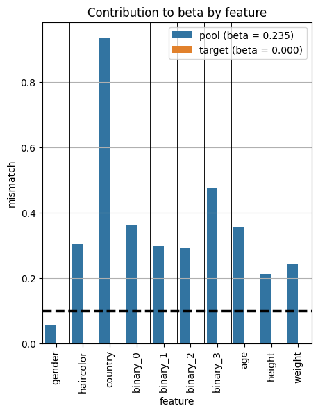
# Plot the standardized mean difference for each feature
from pybalance.utils import BetaBalance
bc = BetaBalance(m, standardize_difference=True)
fig = plot_per_feature_loss(m, bc)
[13]:
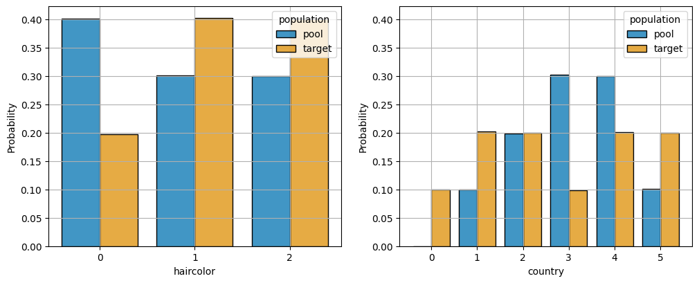
fig = plot_categoric_features(m, cumulative=False, palette='colorblind', include_binary=False)
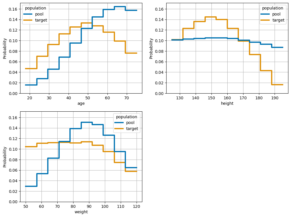
[14]:
fig = plot_numeric_features(m, bins=10, cumulative=False, palette='colorblind')
[15]:
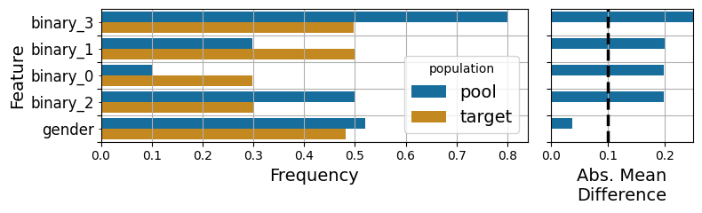
fig = plot_binary_features(m, palette='colorblind', orient_horizontal=False, standardize_difference=False)
/Users/sprivite/src/pybalance/venv/pybalance/lib/python3.9/site-packages/pybalance/visualization/distributions.py:331: UserWarning: set_ticklabels() should only be used with a fixed number of ticks, i.e. after set_ticks() or using a FixedLocator.
  plt.gca().set_yticklabels([""] * len(labels), minor=True)