Fitting a biphasic dose-reponse model
Source:vignettes/articles/Advanced_Fitting-a-biphasic-dose-reponse-model.Rmd
Advanced_Fitting-a-biphasic-dose-reponse-model.RmdThis article is to reproduce the biphasic dose responses demonstrated in the Stackoverflow post and in the supplementing material
library(drcHelper)
#> Loading required package: drc
#> Loading required package: MASS
#> Loading required package: drcData
#>
#> 'drc' has been loaded.
#> Please cite R and 'drc' if used for a publication,
#> for references type 'citation()' and 'citation('drc')'.
#>
#> Attaching package: 'drc'
#> The following objects are masked from 'package:stats':
#>
#>     gaussian, getInitial
library(drc)
Stackoverflow
dat <- structure(list(Concn = c(1e-05, 4e-06, 1.5e-06, 7.5e-07, 2.5e-07,
1e-07, 3.75e-08, 1.63e-08, 6.25e-09, 2.5e-09, 1.06e-09, 4.06e-10,
1.56e-10, 6.25e-11, 2.66e-11, 1.09e-11), CompoundX = c(0.309967,
0.239756, 0.924346, 1.409483, 2.128796, 2.407227, 2.300768, 1.826203,
0.978104, 0.483403, 0.235191, 0.115721, 0.06902, 0.031384, 0.023007,
0.003956), CompoundX.2 = c(0.28848, 0.386004, 0.924336, 1.310479,
2.007222, 2.371517, 2.203162, 1.654133, 1.06907, 0.473238, 0.251971,
0.114867, 0.053681, 0.054416, 0.028945, 0.020866)), class = "data.frame", row.names = c(NA,
-16L))

m0<-drm(CompoundX~log(Concn), data = dat, fct = gaussian())
summary(m0)
#>
#> Model fitted: Gaussian (5 parms)
#>
#> Parameter estimates:
#>
#>                 Estimate Std. Error   t-value   p-value
#> b:(Intercept)   2.039632   0.082528   24.7144 5.461e-11 ***
#> c:(Intercept)   0.027623   0.038466    0.7181    0.4877
#> d:(Intercept)   2.437808   0.064117   38.0214 5.036e-13 ***
#> e:(Intercept) -16.270101   0.044150 -368.5165 < 2.2e-16 ***
#> f:(Intercept)   2.152055   0.195211   11.0242 2.767e-07 ***
#> ---
#> Signif. codes:  0 '***' 0.001 '**' 0.01 '*' 0.05 '.' 0.1 ' ' 1
#>
#> Residual standard error:
#>
#>  0.07611998 (11 degrees of freedom)


plot(m0, type = "all", col= "black", log = "")
#> Warning in min(dose[dose > 0]): no non-missing arguments to min; returning Inf
Scatter plot and fitted curves of a biphasic dose-response model
Defining
data(metaldata)
#Make a subset with the Zn data
Zn <- metaldata[metaldata$metal=="Zn",]
Zn
#>    metal    conc         IR
#> 1     Zn  0.0369  0.9142857
#> 2     Zn  0.0369  0.9756098
#> 3     Zn  0.0369  0.8974359
#> 4     Zn  0.0925  0.9523810
#> 5     Zn  0.0925  0.8780488
#> 6     Zn  0.0925  1.1666667
#> 7     Zn  0.1859  0.9523810
#> 8     Zn  0.1859  1.1707317
#> 9     Zn  0.1859  1.2115385
#> 10    Zn  0.5693  1.7523810
#> 11    Zn  0.5693  1.6585366
#> 12    Zn  0.5693  1.7948718
#> 13    Zn  0.9684  5.9809524
#> 14    Zn  0.9684  4.6341463
#> 15    Zn  0.9684  4.8461538
#> 16    Zn  1.3836 14.2857143
#> 17    Zn  1.3836 19.7073171
#> 18    Zn  1.3836 22.7051282
#> 19    Zn  1.4472 43.9500000
#> 20    Zn  1.4472 44.0869565
#> 21    Zn  1.4472 43.2000000
#> 22    Zn  2.0371 67.1238095
#> 23    Zn  2.0371 74.0975610
#> 24    Zn  2.0371 86.0192308
#> 25    Zn  3.2111 31.1619048
#> 26    Zn  3.2111 61.2195122
#> 27    Zn  3.2111 64.6153846
#> 28    Zn  4.4946  3.8857143
#> 29    Zn  4.4946  4.8292683
#> 30    Zn  4.4946  5.3846154
#> 31    Zn 10.7532  0.3428571
#> 32    Zn 10.7532  0.5853659
#> 33    Zn 10.7532  0.6730769
#Fitting biphasic dose-response profiles
#gaussian function
Zn.gau <- drm(IR~conc, data=Zn, fct=gaussian(), na.action=na.omit)
summary(Zn.gau)
#>
#> Model fitted: Gaussian (5 parms)
#>
#> Parameter estimates:
#>
#>                 Estimate Std. Error  t-value   p-value
#> b:(Intercept)  0.8861307  0.0093682  94.5893 < 2.2e-16 ***
#> c:(Intercept)  2.1659895  1.2820509   1.6895    0.1022
#> d:(Intercept) 75.7461755  3.3920022  22.3308 < 2.2e-16 ***
#> e:(Intercept)  2.3418279  0.0086316 271.3077 < 2.2e-16 ***
#> f:(Intercept) 13.8801613  2.8981117   4.7894 4.933e-05 ***
#> ---
#> Signif. codes:  0 '***' 0.001 '**' 0.01 '*' 0.05 '.' 0.1 ' ' 1
#>
#> Residual standard error:
#>
#>  5.87511 (28 degrees of freedom)
#Model checking
plot(fitted(Zn.gau), residuals(Zn.gau), ylim = c(-20, 20))
# Gaussian function with Box-Cox transform
Zn.gau2 <- drm(IR~conc, data=Zn, fct=gaussian(), na.action=na.omit, bcVal = 0, bcAdd = 10)
summary(Zn.gau2)
#>
#> Model fitted: Gaussian (5 parms)
#>
#> Parameter estimates:
#>
#>                Estimate Std. Error t-value   p-value
#> b:(Intercept)  0.793259   0.075520 10.5040 3.215e-11 ***
#> c:(Intercept)  1.613775   0.500908  3.2217  0.003223 **
#> d:(Intercept) 81.080825  10.982113  7.3830 4.859e-08 ***
#> e:(Intercept)  2.422227   0.042576 56.8923 < 2.2e-16 ***
#> f:(Intercept)  3.115795   0.624967  4.9855 2.885e-05 ***
#> ---
#> Signif. codes:  0 '***' 0.001 '**' 0.01 '*' 0.05 '.' 0.1 ' ' 1
#>
#> Residual standard error:
#>
#>  0.17677 (28 degrees of freedom)
#>
#> Non-normality/heterogeneity adjustment through Box-Cox transformation
#>
#> Specified lambda: 0
#Model checking
plot(fitted(Zn.gau2), residuals(Zn.gau2), ylim = c(-0.4, 0.4))
#lgaussian function
Zn.lgau <- drm(IR~conc, data=Zn, fct=lgaussian(), na.action=na.omit)
summary(Zn.lgau)
#>
#> Model fitted: Log-Gaussian (5 parms)
#>
#> Parameter estimates:
#>
#>                 Estimate Std. Error  t-value   p-value
#> b:(Intercept)  0.4013399  0.0064603  62.1238 < 2.2e-16 ***
#> c:(Intercept)  2.1660776  1.2820555   1.6895    0.1022
#> d:(Intercept) 75.7466002  3.3919724  22.3311 < 2.2e-16 ***
#> e:(Intercept)  2.1746086  0.0128388 169.3773 < 2.2e-16 ***
#> f:(Intercept)  9.1065547  1.8772570   4.8510 4.168e-05 ***
#> ---
#> Signif. codes:  0 '***' 0.001 '**' 0.01 '*' 0.05 '.' 0.1 ' ' 1
#>
#> Residual standard error:
#>
#>  5.87511 (28 degrees of freedom)
#Model checking
plot(fitted(Zn.lgau), residuals(Zn.lgau), ylim = c(-20, 20))
# lgaussian function with Box-Cox transform
Zn.lgau2 <- drm(IR~conc, data=Zn, fct=lgaussian(), na.action=na.omit, bcVal = 0, bcAdd = 10)
summary(Zn.lgau2)
#>
#> Model fitted: Log-Gaussian (5 parms)
#>
#> Parameter estimates:
#>
#>                Estimate Std. Error t-value   p-value
#> b:(Intercept)  0.351996   0.048207  7.3018 5.978e-08 ***
#> c:(Intercept)  1.475965   0.597634  2.4697  0.019884 *
#> d:(Intercept) 80.099960   9.894407  8.0955 8.170e-09 ***
#> e:(Intercept)  2.245102   0.043678 51.4011 < 2.2e-16 ***
#> f:(Intercept)  2.662339   0.829132  3.2110  0.003312 **
#> ---
#> Signif. codes:  0 '***' 0.001 '**' 0.01 '*' 0.05 '.' 0.1 ' ' 1
#>
#> Residual standard error:
#>
#>  0.1698429 (28 degrees of freedom)
#>
#> Non-normality/heterogeneity adjustment through Box-Cox transformation
#>
#> Specified lambda: 0
#Model checking
plot(fitted(Zn.lgau2), residuals(Zn.lgau2), ylim = c(-0.4, 0.4))
#plot the models fitted
plot(Zn.gau, type = "obs", col= "black", log = "")
plot(Zn.gau, type = "none", add = TRUE, col = "red")
plot(Zn.gau2, type = "none", add = TRUE, col = "yellow")
plot(Zn.lgau, type = "none", add = TRUE, col = "blue")
plot(Zn.lgau2, type = "none", add = TRUE, col = "green")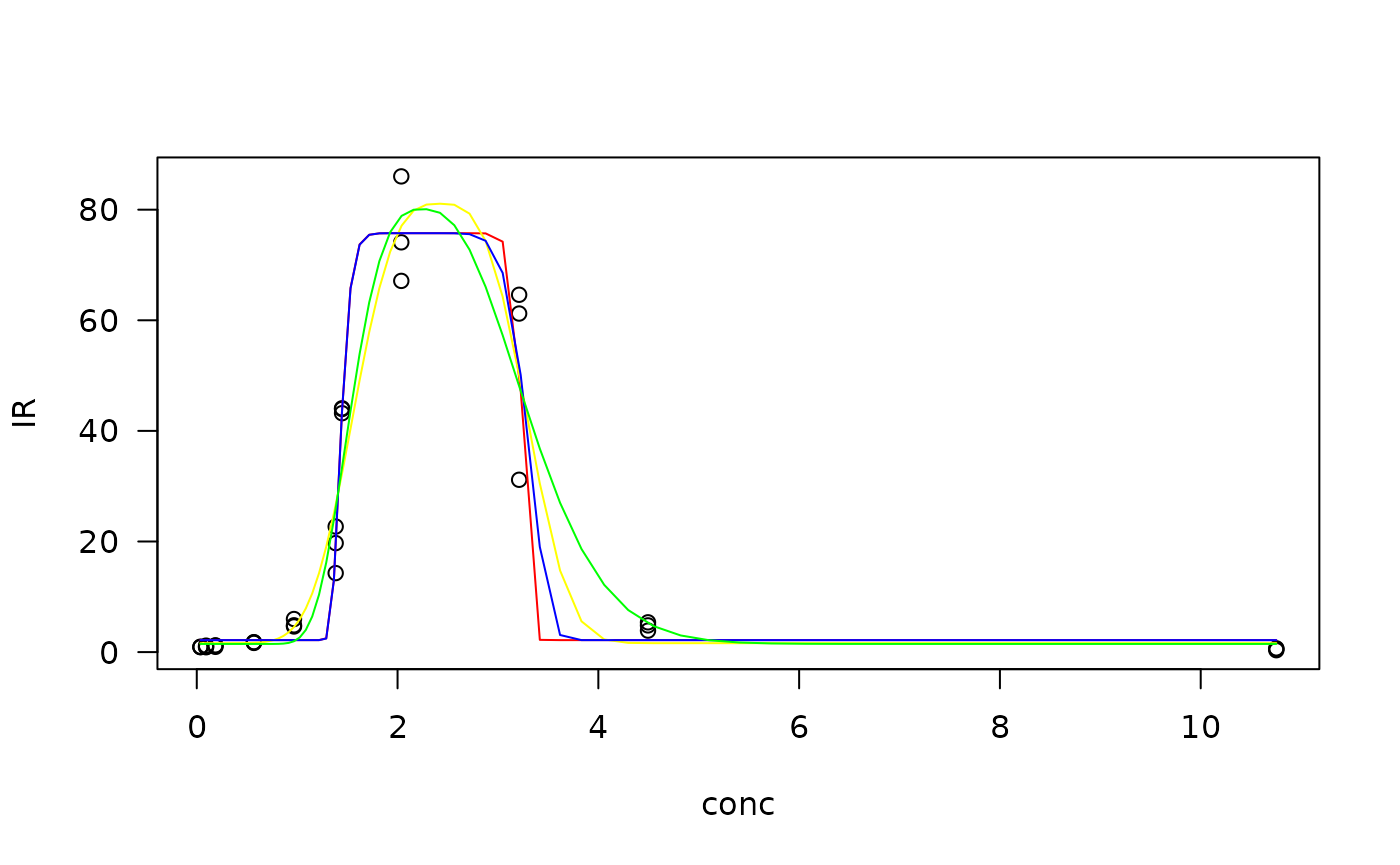
#Effective doses (EDp) calculation
ED(Zn.lgau2, 50, interval = "delta")
#>
#> Estimated effective doses
#>
#>        Estimate Std. Error   Lower   Upper
#> e:1:50  3.34241    0.18363 2.96627 3.71855
ED(Zn.lgau2, -50, interval = "delta", bound = FALSE)
#>
#> Estimated effective doses
#>
#>         Estimate Std. Error    Lower    Upper
#> e:1:-50 1.508038   0.082849 1.338329 1.677746
ED(Zn.lgau2, 99.9,interval = "delta")
#>
#> Estimated effective doses
#>
#>          Estimate Std. Error   Lower   Upper
#> e:1:99.9  2.32300    0.10458 2.10877 2.53723

#Make a subset with the Cd data
Cd <- metaldata[metaldata$metal=="Cd",]
Cd
#>    metal    conc         IR
#> 34    Cd  0.1004  0.8761905
#> 35    Cd  0.1004  0.8906250
#> 36    Cd  0.1004  0.8194444
#> 37    Cd  0.2517  0.8000000
#> 38    Cd  0.2517  1.1718750
#> 39    Cd  0.2517  1.0138889
#> 40    Cd  0.5055  1.0285714
#> 41    Cd  0.5055  1.0312500
#> 42    Cd  0.5055  1.0416667
#> 43    Cd  1.5398  2.5523810
#> 44    Cd  1.5398  2.8593750
#> 45    Cd  1.5398  2.0694444
#> 46    Cd  2.6010 18.1333333
#> 47    Cd  2.6010 17.5781250
#> 48    Cd  2.6010 30.6111111
#> 49    Cd  3.6856 39.5428571
#> 50    Cd  3.6856 41.8333333
#> 51    Cd  5.3508 55.7714286
#> 52    Cd  5.3508 47.1944444
#> 53    Cd  8.2131 35.9238095
#> 54    Cd  8.2131 40.0312500
#> 55    Cd  8.2131 35.2638889
#> 56    Cd 11.1672 15.3523810
#> 57    Cd 11.1672 25.1250000
#> 58    Cd 11.1672 20.8888889
#> 59    Cd 23.6932  1.6000000
#> 60    Cd 23.6932  2.2968750
#> 61    Cd 23.6932  1.8750000
#Fitting biphasic dose-response profiles
#gaussian function
Cd.gau <- drm(IR~conc, data=Cd, fct=gaussian(), na.action=na.omit)
summary(Cd.gau)
#>
#> Model fitted: Gaussian (5 parms)
#>
#> Parameter estimates:
#>
#>                Estimate Std. Error t-value p-value
#> b:(Intercept)  4.079689   0.115139 35.4326 < 2e-16 ***
#> c:(Intercept)  1.283627   1.275138  1.0067 0.32457
#> d:(Intercept) 42.981885   1.907644 22.5314 < 2e-16 ***
#> e:(Intercept)  6.850150   0.070015 97.8387 < 2e-16 ***
#> f:(Intercept)  7.805005   3.237173  2.4111 0.02429 *
#> ---
#> Signif. codes:  0 '***' 0.001 '**' 0.01 '*' 0.05 '.' 0.1 ' ' 1
#>
#> Residual standard error:
#>
#>  4.4849 (23 degrees of freedom)
#Model checking
plot(fitted(Cd.gau), residuals(Cd.gau), ylim = c(-10, 10))
#Gaussian function with Box-Cox transform
Cd.gau2 <- drm(IR~conc, data=Cd, fct=gaussian(), na.action=na.omit, bcVal = 0, bcAdd = 10)
summary(Cd.gau2)
#>
#> Model fitted: Gaussian (5 parms)
#>
#> Parameter estimates:
#>
#>                Estimate Std. Error  t-value   p-value
#> b:(Intercept)  4.056422   0.090069  45.0368 < 2.2e-16 ***
#> c:(Intercept)  1.202271   0.352358   3.4121  0.002388 **
#> d:(Intercept) 42.700145   2.340528  18.2438 3.551e-15 ***
#> e:(Intercept)  6.851570   0.053432 128.2305 < 2.2e-16 ***
#> f:(Intercept)  7.234677   1.057973   6.8382 5.667e-07 ***
#> ---
#> Signif. codes:  0 '***' 0.001 '**' 0.01 '*' 0.05 '.' 0.1 ' ' 1
#>
#> Residual standard error:
#>
#>  0.1088791 (23 degrees of freedom)
#>
#> Non-normality/heterogeneity adjustment through Box-Cox transformation
#>
#> Specified lambda: 0
#Model checking
plot(fitted(Cd.gau2), residuals(Cd.gau2), ylim = c(-0.2, 0.2))
#lgaussian function
Cd.lgau <- drm(IR~conc, data=Cd, fct=lgaussian(), na.action=na.omit)
summary(Cd.lgau)
#>
#> Model fitted: Log-Gaussian (5 parms)
#>
#> Parameter estimates:
#>
#>                Estimate Std. Error t-value   p-value
#> b:(Intercept)  0.544683   0.032578 16.7195 2.308e-14 ***
#> c:(Intercept)  0.806563   0.920847  0.8759    0.3901
#> d:(Intercept) 51.009281   2.143174 23.8008 < 2.2e-16 ***
#> e:(Intercept)  5.315768   0.093498 56.8542 < 2.2e-16 ***
#> f:(Intercept)  2.105116   0.261655  8.0454 3.892e-08 ***
#> ---
#> Signif. codes:  0 '***' 0.001 '**' 0.01 '*' 0.05 '.' 0.1 ' ' 1
#>
#> Residual standard error:
#>
#>  3.086809 (23 degrees of freedom)
#Model checking
plot(fitted(Cd.lgau), residuals(Cd.lgau), ylim = c(-6, 6), xlim = c(0, 50)) 
#lgaussian function with Box-Cox transform
Cd.lgau2 <- drm(IR~conc, data=Cd, fct=lgaussian(), na.action=na.omit, bcVal = 0, bcAdd = 10)
summary(Cd.lgau2)
#>
#> Model fitted: Log-Gaussian (5 parms)
#>
#> Parameter estimates:
#>
#>                Estimate Std. Error t-value   p-value
#> b:(Intercept)  0.562495   0.039451 14.2581 6.590e-13 ***
#> c:(Intercept)  1.039686   0.314707  3.3037  0.003103 **
#> d:(Intercept) 49.728622   3.290085 15.1147 1.950e-13 ***
#> e:(Intercept)  5.340496   0.093375 57.1938 < 2.2e-16 ***
#> f:(Intercept)  2.358463   0.293418  8.0379 3.955e-08 ***
#> ---
#> Signif. codes:  0 '***' 0.001 '**' 0.01 '*' 0.05 '.' 0.1 ' ' 1
#>
#> Residual standard error:
#>
#>  0.09005292 (23 degrees of freedom)
#>
#> Non-normality/heterogeneity adjustment through Box-Cox transformation
#>
#> Specified lambda: 0
#Model checking
plot(fitted(Cd.lgau2), residuals(Cd.lgau2), ylim = c(-0.3, 0.3))
#plot the models fitted
plot(Cd.gau, type = "obs", col= "black", log = "", ylim = c(0, 60))
plot(Cd.gau, type = "none", add = TRUE, col = "red")
plot(Cd.gau2, type = "none", add = TRUE, col = "yellow")
plot(Cd.lgau, type = "none", add = TRUE, col = "blue")
plot(Cd.lgau2, type = "none", add = TRUE, col = "green")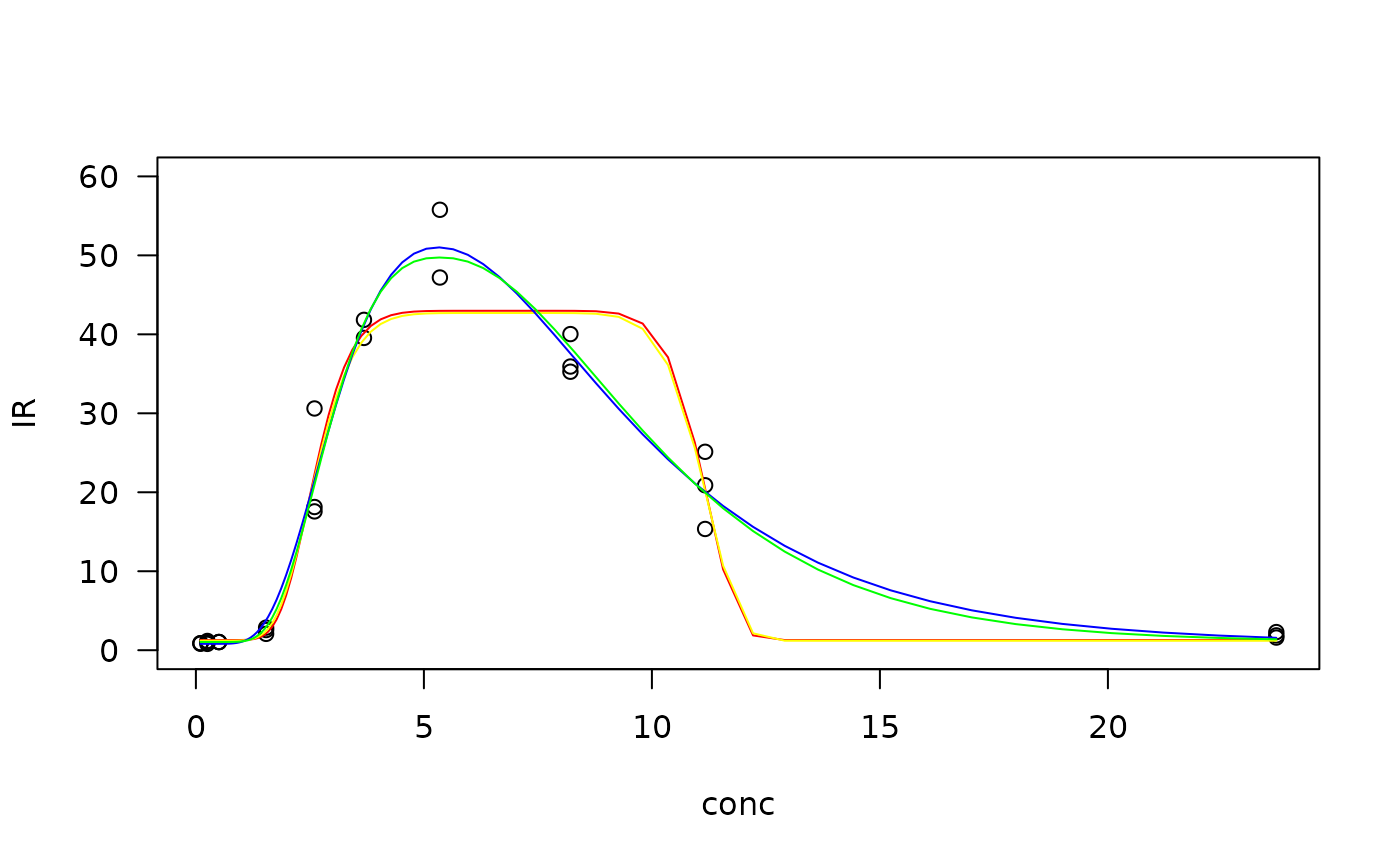
#Effective doses (D(p)) calculation
ED(Cd.lgau2, -50, interval = "delta", bound = FALSE)
#>
#> Estimated effective doses
#>
#>         Estimate Std. Error   Lower   Upper
#> e:1:-50  2.79902    0.10714 2.57737 3.02066
ED(Cd.lgau2, 99.9,interval = "delta")
#>
#> Estimated effective doses
#>
#>          Estimate Std. Error   Lower   Upper
#> e:1:99.9  5.56039    0.11333 5.32594 5.79483
ED(Cd.lgau2, 50,interval = "delta")
#>
#> Estimated effective doses
#>
#>        Estimate Std. Error    Lower    Upper
#> e:1:50 10.18961    0.39005  9.38273 10.99649

# Make a subset with the ZnCd data
ZnCd <- metaldata[metaldata$metal=="ZnCd",]
ZnCd
#>     metal      conc        IR
#> 326  ZnCd 0.9671179 13.276596
#> 327  ZnCd 0.9671179 11.744681
#> 328  ZnCd 0.9671179 11.404255
#> 329  ZnCd 0.9671179 11.574468
#> 330  ZnCd 1.9969972 42.808511
#> 331  ZnCd 1.9969972 41.744681
#> 332  ZnCd 1.9969972 40.808511
#> 333  ZnCd 1.9969972 40.255319
#> 334  ZnCd 4.1971350 25.914894
#> 335  ZnCd 4.1971350 23.914894
#> 336  ZnCd 4.1971350 23.361702
#> 337  ZnCd 4.1971350 23.489362
#> 338  ZnCd 5.9729887  9.574468
#> 339  ZnCd 5.9729887  9.702128
#> 340  ZnCd 5.9729887  9.914894
#> 341  ZnCd 5.9729887  9.489362
#> 342  ZnCd 9.1994126  1.787234
#> 343  ZnCd 9.1994126  1.361702
#> 344  ZnCd 9.1994126  1.446809
#> 345  ZnCd 9.1994126  1.702128

#gaussian function
ZnCd.gau <- drm(IR~conc, data=ZnCd, fct=gaussian(), na.action=na.omit)
summary(ZnCd.gau)
#> Warning in sqrt(diag(varMat)): NaNs produced
#>
#> Model fitted: Gaussian (5 parms)
#>
#> Parameter estimates:
#>
#>                 Estimate Std. Error  t-value   p-value
#> b:(Intercept) 8.3214e-03        NaN      NaN       NaN
#> c:(Intercept) 2.2642e+00 1.1019e+00   2.0548   0.05774 .
#> d:(Intercept) 1.0820e+03        NaN      NaN       NaN
#> e:(Intercept) 2.8890e+00 2.3294e-02 124.0227 < 2.2e-16 ***
#> f:(Intercept) 4.0544e-01 1.6222e-02  24.9934 1.222e-13 ***
#> ---
#> Signif. codes:  0 '***' 0.001 '**' 0.01 '*' 0.05 '.' 0.1 ' ' 1
#>
#> Residual standard error:
#>
#>  2.120518 (15 degrees of freedom)
#Model checking
plot(fitted(ZnCd.gau), residuals(ZnCd.gau))
#> Warning in sqrt(diag(varMat)): NaNs produced
#> Warning in sqrt(diag(varMat)): NaNs produced
#Gaussian function with Box-Cox transform
ZnCd.gau2 <- drm(IR~conc, data=ZnCd, fct=gaussian(), na.action=na.omit, bcVal = 0, bcAdd = 10)
summary(ZnCd.gau2)
#>
#> Model fitted: Gaussian (5 parms)
#>
#> Parameter estimates:
#>
#>                 Estimate Std. Error t-value   p-value
#> b:(Intercept)   0.040953   0.033257  1.2314   0.23712
#> c:(Intercept)   0.579361   1.245712  0.4651   0.64855
#> d:(Intercept) 329.177040 137.561825  2.3929   0.03024 *
#> e:(Intercept)   2.899653   0.048979 59.2017 < 2.2e-16 ***
#> f:(Intercept)   0.475406   0.075453  6.3007 1.422e-05 ***
#> ---
#> Signif. codes:  0 '***' 0.001 '**' 0.01 '*' 0.05 '.' 0.1 ' ' 1
#>
#> Residual standard error:
#>
#>  0.1078937 (15 degrees of freedom)
#>
#> Non-normality/heterogeneity adjustment through Box-Cox transformation
#>
#> Specified lambda: 0
#Model checking
plot(fitted(ZnCd.gau2), residuals(ZnCd.gau2), ylim = c(-0.15, 0.15))
#lgaussian function
ZnCd.lgau <- drm(IR~conc, data=ZnCd, fct=lgaussian(), na.action=na.omit)
summary(ZnCd.lgau)
#>
#> Model fitted: Log-Gaussian (5 parms)
#>
#> Parameter estimates:
#>
#>                Estimate Std. Error  t-value   p-value
#> b:(Intercept)  0.555663   0.015419  36.0386 4.972e-16 ***
#> c:(Intercept) -0.274800   1.032831  -0.2661    0.7938
#> d:(Intercept) 42.904780   0.747360  57.4084 < 2.2e-16 ***
#> e:(Intercept)  2.321479   0.018413 126.0780 < 2.2e-16 ***
#> f:(Intercept)  2.028462   0.164444  12.3353 2.963e-09 ***
#> ---
#> Signif. codes:  0 '***' 0.001 '**' 0.01 '*' 0.05 '.' 0.1 ' ' 1
#>
#> Residual standard error:
#>
#>  0.834502 (15 degrees of freedom)
#Model checking
plot(fitted(ZnCd.lgau), residuals(ZnCd.lgau), ylim = c(-2, 2))
#lgaussian function with Box-Cox transform
ZnCd.lgau2 <- drm(IR~conc, data=ZnCd, fct=lgaussian(), na.action=na.omit, bcVal = 0, bcAdd = 10)
summary(ZnCd.lgau2)
#>
#> Model fitted: Log-Gaussian (5 parms)
#>
#> Parameter estimates:
#>
#>                Estimate Std. Error  t-value   p-value
#> b:(Intercept)  0.555188   0.015215  36.4897 4.508e-16 ***
#> c:(Intercept) -0.290451   0.583670  -0.4976     0.626
#> d:(Intercept) 42.910857   0.943991  45.4568 < 2.2e-16 ***
#> e:(Intercept)  2.321820   0.012425 186.8676 < 2.2e-16 ***
#> f:(Intercept)  2.024344   0.134982  14.9971 1.947e-10 ***
#> ---
#> Signif. codes:  0 '***' 0.001 '**' 0.01 '*' 0.05 '.' 0.1 ' ' 1
#>
#> Residual standard error:
#>
#>  0.02654068 (15 degrees of freedom)
#>
#> Non-normality/heterogeneity adjustment through Box-Cox transformation
#>
#> Specified lambda: 0
#Model checking
plot(fitted(ZnCd.lgau2), residuals(ZnCd.lgau2), ylim = c(-0.06, 0.06))
#plot the models fitted
plot(ZnCd.gau, type = "obs", col= "black", ylim = c(0, 300))
plot(ZnCd.gau, type = "none", add = TRUE, col = "red")
plot(ZnCd.gau2, type = "none", add = TRUE, col = "yellow")
plot(ZnCd.lgau, type = "none", add = TRUE, col = "blue")
plot(ZnCd.lgau2, type = "none", add = TRUE, col = "green")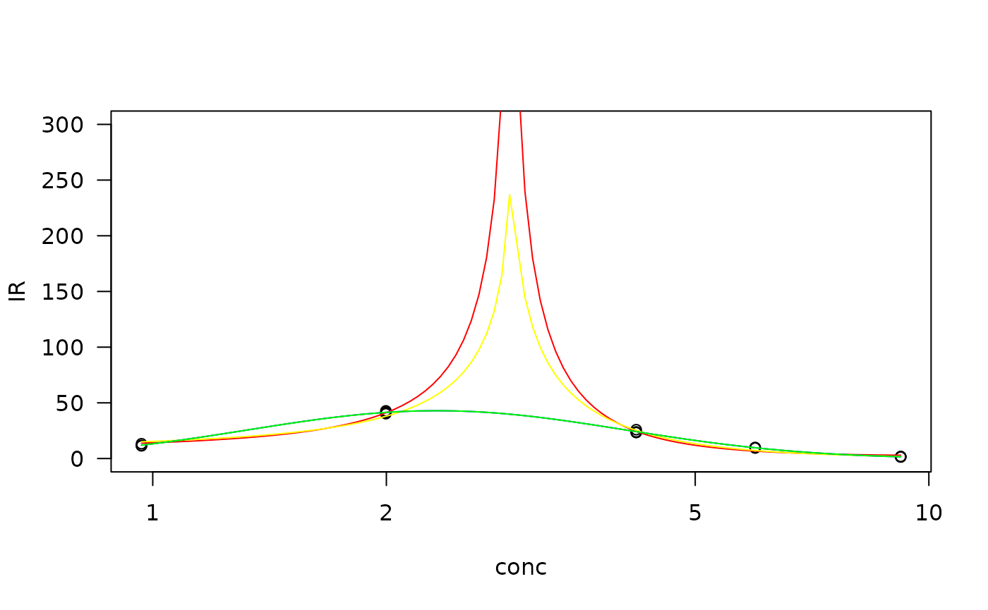
#Effective doses (D(p)) calculation
ED(ZnCd.lgau2, -50, interval = "delta", bound = FALSE)
#>
#> Estimated effective doses
#>
#>         Estimate Std. Error    Lower    Upper
#> e:1:-50 1.209189   0.014632 1.178001 1.240377
ED(ZnCd.lgau2, 99.9,interval = "delta")
#>
#> Estimated effective doses
#>
#>          Estimate Std. Error    Lower    Upper
#> e:1:99.9 2.382456   0.015367 2.349703 2.415210
ED(ZnCd.lgau2, 50,interval = "delta")
#>
#> Estimated effective doses
#>
#>        Estimate Std. Error    Lower    Upper
#> e:1:50 4.458236   0.053948 4.343248 4.573224
# Additivity predictions and departures from additivity
indicesFct(0.355,list(ZnCd.lgau2, Zn.lgau2, Cd.lgau2), c(-0.2, -0.5, -1, -2, -5, -10, -20, -30, -40, -50, -60, -70, -80, -90, -99, 99, 80, 70, 60, 50, 40, 30, 20, 10, 5, 2, 1, 0.5, 0.2))
#plot CIx
plotFACI(0.355,list(ZnCd.lgau2, Zn.lgau2, Cd.lgau2), "x", ylim = c(-0.2, 2.2), faValues = c(-10, -20, -30, -40, -50, -60, -70, -80, -90, -99, 99, 90, 80, 70, 60, 50, 40, 30, 20, 10), showPoints = TRUE)
title("Combination index for x axis")

#plot CIy
plotFACI(0.355,list(ZnCd.lgau2, Zn.lgau2, Cd.lgau2), "y", ylim = c(-0.2, 2.2), faValues = c(-10, -20, -30, -40, -50, -60, -70, -80, -90, -99, 99, 90, 80, 70, 60, 50, 40, 30, 20, 10), showPoints = TRUE)
title("Combination index for y axis")
References
- Martin-Betancor K, Ritz C, Fernández-Piñas F, Leganés F, Rodea-Palomares I. Defining an additivity framework for mixture research in inducible whole-cell biosensors. Sci Rep. 2015 Nov 26;5:17200. doi: 10.1038/srep17200. PMID: 26606975; PMCID: PMC4660423.
- https://stackoverflow.com/questions/72472432/how-to-fit-a-biphasic-dose-response-curve-using-r