In this vignette, we demonstrate how to use the {drcHelper} package to create tables and graphs for inclusion in a dose-response analysis report. While the functions were developed some time ago and may not represent the most elegant solutions, they are functional. We welcome any suggestions for improvement.
Preliminary Summary
data("dat_medium")
dat_medium <- dat_medium %>% mutate(Treatment=factor(Dose,levels=unique(Dose)))
dat_medium$Response[dat_medium$Response < 0] <- 0
prelimPlot3(dat_medium)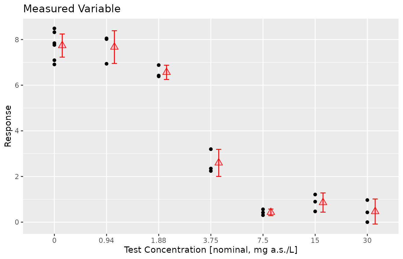
prelimSummary(dat_medium) %>% knitr::kable(.,digits = 3)| Dose | Mean | SD | % Inhibition | CV |
|---|---|---|---|---|
| 0.00 | 7.736 | 0.635 | 0.000 | 8.203 |
| 0.94 | 7.669 | 0.633 | 0.858 | 8.259 |
| 1.88 | 6.563 | 0.275 | 15.161 | 4.197 |
| 3.75 | 2.596 | 0.524 | 66.440 | 20.175 |
| 7.50 | 0.429 | 0.128 | 94.456 | 29.865 |
| 15.00 | 0.859 | 0.372 | 88.892 | 43.296 |
| 30.00 | 0.465 | 0.485 | 93.984 | 104.162 |
Fitting multiple models and rank them.
mod <- drm(Response~Dose,data=dat_medium,fct=LL.3())
fctList <- list(LN.4(),LL.4(),W1.3(),LL2.2())
# plot(mod,type="all")
res <- mselect.plus(mod,fctList = fctList )
modList <- res$modList
res$Comparison
#>          logLik        IC  Lack of fit    Res var
#> LN.4  -14.65361  39.30722 6.118094e-01  0.2382532
#> LL.4  -14.94568  39.89136 5.241523e-01  0.2441232
#> LL.3  -19.24379  46.48759 6.848925e-02  0.3326394
#> W1.3  -20.46060  48.92121 3.233853e-02  0.3681387
#> LL2.2 -70.78500 147.57000 5.059273e-17 23.2867452

drcCompare(modRes=res)
#>          logLik        IC  Lack of fit    Res var Certainty_Protection
#> LN.4  -14.65361  39.30722 6.118094e-01  0.2382532                 High
#> LL.4  -14.94568  39.89136 5.241523e-01  0.2441232                 High
#> LL.3  -19.24379  46.48759 6.848925e-02  0.3326394                 High
#> W1.3  -20.46060  48.92121 3.233853e-02  0.3681387               Medium
#> LL2.2 -70.78500 147.57000 5.059273e-17 23.2867452                  Low
#>       Steepness No Effect p-val
#> LN.4     Medium               0
#> LL.4     Medium               0
#> LL.3     Medium               0
#> W1.3     Medium               0
#> LL2.2     Steep               1
library(purrr)
edResTab <- mselect.ED(modList = modList,respLev = c(10,20,50),trend="Decrease",CI="inv")
edResTab
#>      .id Estimate Std. Error    Lower    Upper        NW      Rating    EC
#> 1   LN.4 1.700984         NA 1.473332 1.981769 0.2989078        Good EC 10
#> 2   LN.4 2.067640         NA 1.826100 2.313691 0.2358199        Good EC 20
#> 3   LN.4 3.032169         NA 2.791669 3.273468 0.1588960   Excellent EC 50
#> 4   LL.4 1.684437         NA 1.432457 2.010475 0.3431521        Good EC 10
#> 5   LL.4 2.085759         NA 1.822344 2.363961 0.2596737        Good EC 20
#> 6   LL.4 3.037357         NA 2.775132 3.288824 0.1691246   Excellent EC 50
#> 7   LL.3 1.577783         NA 1.284085 1.961887 0.4295911        Good EC 10
#> 8   LL.3 2.019241         NA 1.705807 2.342361 0.3152440        Good EC 20
#> 9   LL.3 3.078550         NA 2.783875 3.366535 0.1892644   Excellent EC 50
#> 10  W1.3 1.588648         NA 1.208777 2.089897 0.5546347        Fair EC 10
#> 11  W1.3 2.092308         NA 1.688186 2.490045 0.3832417        Good EC 20
#> 12  W1.3 3.171490         NA 2.862468 3.435822 0.1807837   Excellent EC 50
#> 13 LL2.2       NA         NA       NA       NA        NA Not defined EC 10
#> 14 LL2.2       NA         NA       NA       NA        NA Not defined EC 20
#> 15 LL2.2       NA         NA       NA       NA        NA Not defined EC 50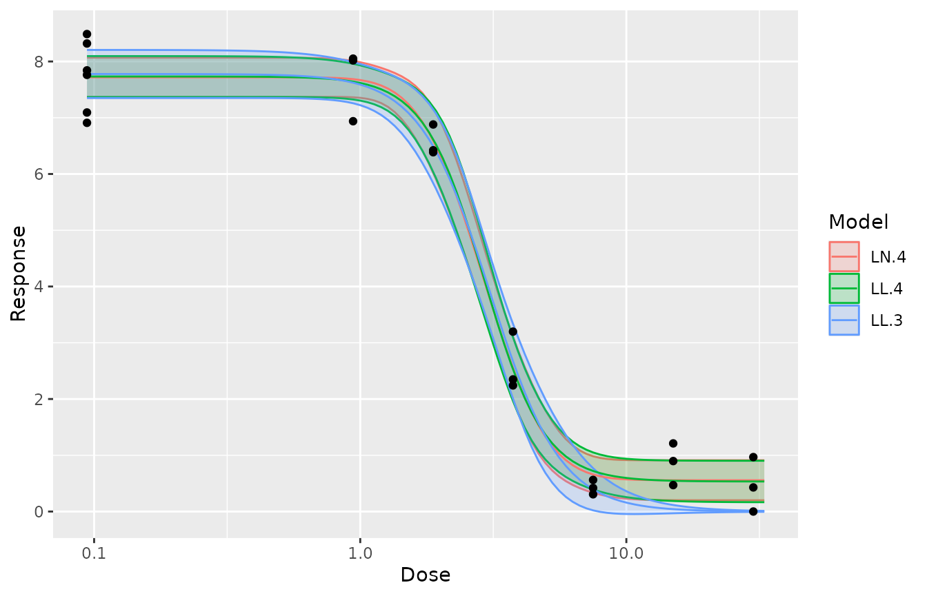
Adding ECx and ECx CI’s to the plots
p1 <- plot.modList(modList[1])
addECxCI(p1,object=modList[[1]],EDres=NULL,trend="Decrease",endpoint="EC", respLev=c(10,20,50),
                     textAjust.x=0.01,textAjust.y=0.3,useObsCtr=FALSE,d0=NULL,textsize = 4,lineheight = 0.5,xmin=0.012)+ ylab("Response Variable [unit]") + xlab("Concentration [µg a.s./L]")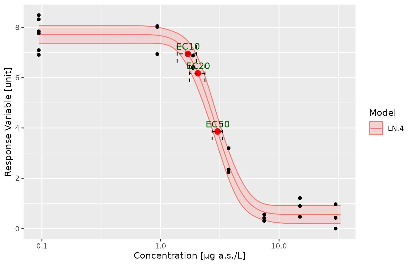
## addECxCI(p)Report ECx
resED <- t(edResTab[1:3, c(2,4,5,6)])
colnames(resED) <- paste("EC", c(10,20,50))
knitr::kable(resED,caption = "Response Variable at day N",digits = 3)| EC 10 | EC 20 | EC 50 | |
|---|---|---|---|
| Estimate | 1.701 | 2.068 | 3.032 |
| Lower | 1.473 | 1.826 | 2.792 |
| Upper | 1.982 | 2.314 | 3.273 |
| NW | 0.299 | 0.236 | 0.159 |
Calculate specific ECx:
mod <-modList[[1]]
edres <- ED.plus(mod,c(5,10,20,50),trend="Decrease")
edres%>%knitr::kable(.,digits = 3)| Estimate | Std. Error | Lower | Upper | |
|---|---|---|---|---|
| EC 5 | 1.449 | 0.157 | 1.122 | 1.777 |
| EC 10 | 1.701 | 0.154 | 1.380 | 2.022 |
| EC 20 | 2.068 | 0.146 | 1.764 | 2.371 |
| EC 50 | 3.032 | 0.147 | 2.725 | 3.340 |
Model Output
| Estimate | Std. Error | t-value | p-value | |
|---|---|---|---|---|
| b:(Intercept) | -2.311 | 0.299 | -7.719 | 0.000 |
| c:(Intercept) | 0.556 | 0.171 | 3.256 | 0.004 |
| d:(Intercept) | 7.719 | 0.168 | 46.004 | 0.000 |
| e:(Intercept) | 2.907 | 0.143 | 20.382 | 0.000 |
Additional Notes
To be written
Dependencies
library(drcHelper)
library(DependenciesGraphs)
dep <- funDependencies("package:drcHelper","ED.plus")
plot(dep)
dep <- funDependencies("package:drcHelper","mselect.ED")
plot(dep)

#dep <- funDependencies("package:drcHelper","mselect.plus")
#plot(dep)

dep <- envirDependencies('package:drcHelper')
plot(dep)