Dunnett's Test for Data with Hierarchical Structure
Source:vignettes/Dunnetts_Test_for_Data_with_Hierarchical_Structure.Rmd
Dunnetts_Test_for_Data_with_Hierarchical_Structure.RmddrcHelper provides a wrapper function
dunnett_test to use the multcomp package to
perform Dunnett tests on both the mixed model for individual data
(ind_model) and the tank-level linear model for aggregated
data (tank_model).
First we simulate a dataset with log-logistic dose-response.
# Let's simulate a single dataset and examine its properties
set.seed(123)

# Simulate dose-response data with specific variance components
sim_data <- simulate_dose_response(
  n_doses = 5,
  dose_range = c(0, 20),
  m_tanks = 4,
  k_individuals = 10,
  var_tank = 6,     # Between-tank variance
  var_individual = 2,  # Within-tank (individual) variance
  include_individuals = TRUE,
  response_function = function(dose) {
    # Simple linear dose-response with threshold at dose 10
    ifelse(dose > 10, 5 + 2 * (dose - 10), 5)
  }
)

# Calculate theoretical ICC
theoretical_icc <- 6 / (6 + 2)  # var_tank / (var_tank + var_individual)
cat("Theoretical ICC:", theoretical_icc, "\n")
#> Theoretical ICC: 0.75

# Examine the data structure
head(sim_data)
#>   Dose Tank Individual Response
#> 1    0    1          1 2.116990
#> 2    0    1          3 3.318858
#> 3    0    4          1 2.985193
#> 4    0    4          3 3.405375
#> 5    0    3          2 7.934101
#> 6    0    2          1 2.787365
str(sim_data)
#> 'data.frame':    200 obs. of  4 variables:
#>  $ Dose      : num  0 0 0 0 0 0 0 0 0 0 ...
#>  $ Tank      : int  1 1 4 4 3 2 2 1 1 4 ...
#>  $ Individual: int  1 3 1 3 2 1 3 2 4 2 ...
#>  $ Response  : num  2.12 3.32 2.99 3.41 7.93 ...

# Visualize the data to see the hierarchical structure
library(ggplot2)

# Plot individual data points with tank means
ggplot(sim_data, aes(x = factor(Dose), y = Response, color = factor(Tank))) +
  geom_jitter(width = 0.2, alpha = 0.5) +
  stat_summary(fun = mean, geom = "point", size = 3) +
  stat_summary(fun = mean, geom = "line", aes(group = factor(Tank))) +
  labs(title = "Dose-Response Data with Hierarchical Structure",
       x = "Dose", y = "Response",
       color = "Tank") +
  theme_minimal()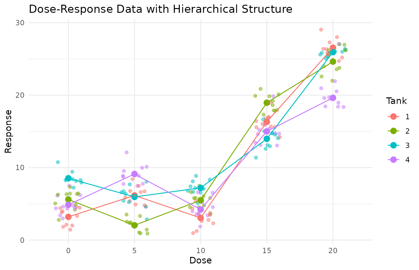
# Calculate observed ICC using a mixed model
library(lme4)
mixed_model <- lmer(Response ~ factor(Dose) + (1|Tank), data = sim_data)
summary(mixed_model)
#> Linear mixed model fit by REML ['lmerMod']
#> Formula: Response ~ factor(Dose) + (1 | Tank)
#>    Data: sim_data
#>
#> REML criterion at convergence: 927.7
#>
#> Scaled residuals:
#>      Min       1Q   Median       3Q      Max
#> -2.22011 -0.64124  0.04355  0.67388  2.79017
#>
#> Random effects:
#>  Groups   Name        Variance Std.Dev.
#>  Tank     (Intercept) 0.424    0.6511
#>  Residual             6.060    2.4617
#> Number of obs: 200, groups:  Tank, 4
#>
#> Fixed effects:
#>                Estimate Std. Error t value
#> (Intercept)      5.5526     0.5074  10.942
#> factor(Dose)5    0.2649     0.5505   0.481
#> factor(Dose)10  -0.5574     0.5505  -1.013
#> factor(Dose)15  10.5100     0.5505  19.093
#> factor(Dose)20  18.6356     0.5505  33.855
#>
#> Correlation of Fixed Effects:
#>             (Intr) fc(D)5 f(D)10 f(D)15
#> factor(Ds)5 -0.542
#> factr(Ds)10 -0.542  0.500
#> factr(Ds)15 -0.542  0.500  0.500
#> factr(Ds)20 -0.542  0.500  0.500  0.500

# Extract variance components
vc <- VarCorr(mixed_model)
tank_var <- as.numeric(vc$Tank)
residual_var <- attr(vc, "sc")^2
observed_icc <- tank_var / (tank_var + residual_var)
cat("Observed ICC:", observed_icc, "\n")
#> Observed ICC: 0.06538746

# Aggregate data to tank level
tank_data <- aggregate(Response ~ Dose + Tank, data = sim_data, FUN = mean)
head(tank_data)
#>   Dose Tank  Response
#> 1    0    1  3.202260
#> 2    5    1  6.156191
#> 3   10    1  3.054297
#> 4   15    1 16.318684
#> 5   20    1 26.548488
#> 6    0    2  5.604946

# Compare individual-level model with tank-level model
# Individual level (mixed model)
ind_model <- lmer(Response ~ factor(Dose) + (1|Tank), data = sim_data)

# Tank level (regular linear model)
tank_model <- lm(Response ~ factor(Dose), data = tank_data)

# Compare model summaries
summary(ind_model)
#> Linear mixed model fit by REML ['lmerMod']
#> Formula: Response ~ factor(Dose) + (1 | Tank)
#>    Data: sim_data
#>
#> REML criterion at convergence: 927.7
#>
#> Scaled residuals:
#>      Min       1Q   Median       3Q      Max
#> -2.22011 -0.64124  0.04355  0.67388  2.79017
#>
#> Random effects:
#>  Groups   Name        Variance Std.Dev.
#>  Tank     (Intercept) 0.424    0.6511
#>  Residual             6.060    2.4617
#> Number of obs: 200, groups:  Tank, 4
#>
#> Fixed effects:
#>                Estimate Std. Error t value
#> (Intercept)      5.5526     0.5074  10.942
#> factor(Dose)5    0.2649     0.5505   0.481
#> factor(Dose)10  -0.5574     0.5505  -1.013
#> factor(Dose)15  10.5100     0.5505  19.093
#> factor(Dose)20  18.6356     0.5505  33.855
#>
#> Correlation of Fixed Effects:
#>             (Intr) fc(D)5 f(D)10 f(D)15
#> factor(Ds)5 -0.542
#> factr(Ds)10 -0.542  0.500
#> factr(Ds)15 -0.542  0.500  0.500
#> factr(Ds)20 -0.542  0.500  0.500  0.500
summary(tank_model)
#>
#> Call:
#> lm(formula = Response ~ factor(Dose), data = tank_data)
#>
#> Residuals:
#>     Min      1Q  Median      3Q     Max
#> -4.5543 -1.2816  0.1967  1.8654  3.3025
#>
#> Coefficients:
#>                Estimate Std. Error t value Pr(>|t|)
#> (Intercept)      5.5526     1.2460   4.456 0.000462 ***
#> factor(Dose)5    0.2649     1.7621   0.150 0.882520
#> factor(Dose)10  -0.5574     1.7621  -0.316 0.756118
#> factor(Dose)15  10.5100     1.7621   5.964 2.59e-05 ***
#> factor(Dose)20  18.6356     1.7621  10.576 2.38e-08 ***
#> ---
#> Signif. codes:  0 '***' 0.001 '**' 0.01 '*' 0.05 '.' 0.1 ' ' 1
#>
#> Residual standard error: 2.492 on 15 degrees of freedom
#> Multiple R-squared:  0.9261, Adjusted R-squared:  0.9063
#> F-statistic: 46.96 on 4 and 15 DF,  p-value: 2.613e-08

# Extract and compare fixed effects
ind_fixed <- fixef(ind_model)
tank_fixed <- coef(tank_model)
Perform Dunnett Test for Different type of Models
Homoscedastic mixed model
# 1. Homoscedastic mixed model (equivalent to ind_model1)
sim_data$Treatment <- factor(sim_data$Dose)
result1 <- dunnett_test(
  data = sim_data,
  response_var = "Response",
  dose_var = "Treatment",  # Using your Treatment factor
  tank_var = "Tank",
  include_random_effect = TRUE,
  variance_structure = "homoscedastic"
)
result1
#> Dunnett Test Results
#> -------------------
#> Model type: Mixed model with homoscedastic errors
#> Control level: 0
#> Alpha level: 0.05
#>
#> Results Table:
#>  comparison   estimate std.error  statistic      p.value  conf.low conf.high
#>       5 - 0  0.2648670  1.762098  0.1503135 9.996387e-01 -4.041493  4.571227
#>      10 - 0 -0.5573896  1.762098 -0.3163216 9.934653e-01 -4.863750  3.748971
#>      15 - 0 10.5099513  1.762098  5.9644545 1.252943e-08  6.203591 14.816312
#>      20 - 0 18.6355902  1.762098 10.5757988 0.000000e+00 14.329230 22.941950
#>  significant
#>        FALSE
#>        FALSE
#>         TRUE
#>         TRUE
#>
#> NOEC Determination:
#> NOEC determined as 10
This is equivalent to
ind_model1 <- lmer(Response ~ Treatment + (1 | Tank),sim_data) ## homoscedastic errors
# Apply Dunnett test to mixed model
ind_dunnett1 <- glht(ind_model1, linfct = mcp(Treatment = "Dunnett"))

s1 <- summary(ind_dunnett1)
result1$results_table$p.value - s1$test$pvalues < 1e-04
#> [1] FALSE FALSE  TRUE  TRUE
Heteroscedastic mixed model
# 2. Heteroscedastic mixed model (equivalent to  mod.nlme)
result2 <- dunnett_test(
  data = sim_data,
  response_var = "Response",
  dose_var = "Treatment",
  tank_var = "Tank",
  include_random_effect = FALSE,
  variance_structure = "heteroscedastic"
)


result2
#> Dunnett Test Results
#> -------------------
#> Model type: Fixed model with heteroscedastic errors
#> Control level: 0
#> Alpha level: 0.05
#>
#> Results Table:
#>  comparison   estimate std.error  statistic   p.value  conf.low conf.high
#>       5 - 0  0.2648670 0.5760347  0.4598109 0.9761703 -1.146160  1.675894
#>      10 - 0 -0.5573896 0.4790326 -1.1635734 0.6085235 -1.730805  0.616026
#>      15 - 0 10.5099513 0.5216412 20.1478537 0.0000000  9.232164 11.787739
#>      20 - 0 18.6355902 0.5972666 31.2014594 0.0000000 17.172554 20.098626
#>  significant
#>        FALSE
#>        FALSE
#>         TRUE
#>         TRUE
#>
#> NOEC Determination:
#> NOEC determined as 10
mod.nlme <- nlme::lme(Response ~ Treatment ,
                       random  = ~ 1 | Tank,
                       weights = varIdent(form= ~1|Treatment),
                       data    = sim_data)
ind_dunnett2 <- glht(mod.nlme, linfct = mcp(Treatment = "Dunnett"))
s2 <- summary(ind_dunnett2)
result2$results_table$p.value - s2$test$pvalues < 1e-05
#> [1]  TRUE FALSE  TRUE  TRUE
result2$results_table$estimate -s2$test$coefficients
#>        5 - 0       10 - 0       15 - 0       20 - 0
#> 9.769963e-15 8.548717e-15 7.105427e-15 7.105427e-15
Homoscedastic fixed effect model
# Tank level (regular linear model)
tank_data$Treatment <- factor(tank_data$Dose)
result3 <- dunnett_test(
  data = tank_data,
  response_var = "Response",
  dose_var = "Treatment",
  tank_var = "Tank",
  include_random_effect = FALSE,
  variance_structure = "homoscedastic"
)
result3
#> Dunnett Test Results
#> -------------------
#> Model type: Fixed model with homoscedastic errors
#> Control level: 0
#> Alpha level: 0.05
#>
#> Results Table:
#>  comparison   estimate std.error  statistic      p.value  conf.low conf.high
#>       5 - 0  0.2648670  1.762097  0.1503135 9.995932e-01 -4.542552  5.072286
#>      10 - 0 -0.5573896  1.762097 -0.3163217 9.927925e-01 -5.364808  4.250029
#>      15 - 0 10.5099513  1.762097  5.9644562 6.506358e-05  5.702533 15.317370
#>      20 - 0 18.6355902  1.762097 10.5758018 4.527548e-09 13.828172 23.443009
#>  significant
#>        FALSE
#>        FALSE
#>         TRUE
#>         TRUE
#>
#> NOEC Determination:
#> NOEC determined as 10
This is equivalent to:
# Tank level (regular linear model)
tank_model <- lm(Response ~ Treatment, data = tank_data)
summary(glht(tank_model,linfct = mcp(Treatment="Dunnett")))
#>
#>   Simultaneous Tests for General Linear Hypotheses
#>
#> Multiple Comparisons of Means: Dunnett Contrasts
#>
#>
#> Fit: lm(formula = Response ~ Treatment, data = tank_data)
#>
#> Linear Hypotheses:
#>             Estimate Std. Error t value Pr(>|t|)
#> 5 - 0 == 0    0.2649     1.7621   0.150    1.000
#> 10 - 0 == 0  -0.5574     1.7621  -0.316    0.993
#> 15 - 0 == 0  10.5100     1.7621   5.964   <1e-04 ***
#> 20 - 0 == 0  18.6356     1.7621  10.576   <1e-04 ***
#> ---
#> Signif. codes:  0 '***' 0.001 '**' 0.01 '*' 0.05 '.' 0.1 ' ' 1
#> (Adjusted p values reported -- single-step method)
Heteroscedastic fixed effect model
result4 <- dunnett_test(
  data = tank_data,
  response_var = "Response",
  dose_var = "Treatment",
  tank_var = NULL,
  include_random_effect = FALSE,
  variance_structure = "heteroscedastic"
)
result4
#> Dunnett Test Results
#> -------------------
#> Model type: Fixed model with heteroscedastic errors
#> Control level: 0
#> Alpha level: 0.05
#>
#> Results Table:
#>  comparison   estimate std.error  statistic      p.value  conf.low conf.high
#>       5 - 0  0.2648670  1.829785  0.1447531 9.997148e-01 -4.216766  4.746500
#>      10 - 0 -0.5573896  1.424783 -0.3912102 9.866375e-01 -4.047064  2.932285
#>      15 - 0 10.5099513  1.548110  6.7888938 2.287759e-11  6.718217 14.301686
#>      20 - 0 18.6355902  1.924281  9.6844412 0.000000e+00 13.922510 23.348670
#>  significant
#>        FALSE
#>        FALSE
#>         TRUE
#>         TRUE
#>
#> NOEC Determination:
#> NOEC determined as 10
This is equivalent to:
library(nlme)
gls0 <- gls(Response ~ Treatment, data=tank_data,weights=varIdent(form= ~1|Treatment))
ind_gls0 <- glht(gls0, linfct = mcp(Treatment = "Dunnett"))

s4 <- summary(ind_gls0)
result4$results_table$estimate -s4$test$coefficients
#>  5 - 0 10 - 0 15 - 0 20 - 0
#>      0      0      0      0
result4$results_table$p.value - s4$test$pvalues < 1e-05
#> [1] TRUE TRUE TRUE TRUE