Using nls to fit arbitrary dose-response models
Source:vignettes/articles/Examples using NLS.Rmd
Examples using NLS.RmdThis article demonstrates how to use nls function to fit a dose-response model, reproduced from ggprism package.
library(drcHelper)
#> Loading required package: drc
#> Loading required package: MASS
#> Loading required package: drcData
#>
#> 'drc' has been loaded.
#> Please cite R and 'drc' if used for a publication,
#> for references type 'citation()' and 'citation('drc')'.
#>
#> Attaching package: 'drc'
#> The following objects are masked from 'package:stats':
#>
#>     gaussian, getInitial
# for the graph
library(ggplot2)
library(ggprism)
library(ggnewscale)

# just for manipulating the data.frame
library(dplyr)
#>
#> Attaching package: 'dplyr'
#> The following object is masked from 'package:MASS':
#>
#>     select
#> The following objects are masked from 'package:stats':
#>
#>     filter, lag
#> The following objects are masked from 'package:base':
#>
#>     intersect, setdiff, setequal, union
library(tidyr)Example Dataset
# construct the data.frame, log10 transform the agonist concentration
# convert the data.frame to long format, then remove any rows with NA
df <- data.frame(
  agonist = c(1e-10, 1e-8, 3e-8, 1e-7, 3e-7, 1e-6, 3e-6, 1e-5, 3e-5, 1e-4, 3e-4),
  ctr1 = c(0, 11, 125, 190, 258, 322, 354, 348, NA, 412, NA),
  ctr2 = c(3, 33, 141, 218, 289, 353, 359, 298, NA, 378, NA),
  ctr3 = c(2, 25, 160, 196, 345, 328, 369, 372, NA, 399, NA),
  trt1 = c(3, NA, 11, 52, 80, 171, 289, 272, 359, 352, 389),
  trt2 = c(5, NA, 25, 55, 77, 195, 230, 333, 306, 320, 338),
  trt3 = c(4, NA, 28, 61, 44, 246, 243, 310, 297, 365, NA)
) %>%
  mutate(log.agonist = log10(agonist)) %>%
  pivot_longer(
    c(-agonist, -log.agonist),
    names_pattern = "(.{3})([0-9])",
    names_to = c("treatment", "rep"),
    values_to = "response"
  ) %>%
  filter(!is.na(response))

head(df)
#> # A tibble: 6 × 5
#>        agonist log.agonist treatment rep   response
#>          <dbl>       <dbl> <chr>     <chr>    <dbl>
#> 1 0.0000000001         -10 ctr       1            0
#> 2 0.0000000001         -10 ctr       2            3
#> 3 0.0000000001         -10 ctr       3            2
#> 4 0.0000000001         -10 trt       1            3
#> 5 0.0000000001         -10 trt       2            5
#> 6 0.0000000001         -10 trt       3            4
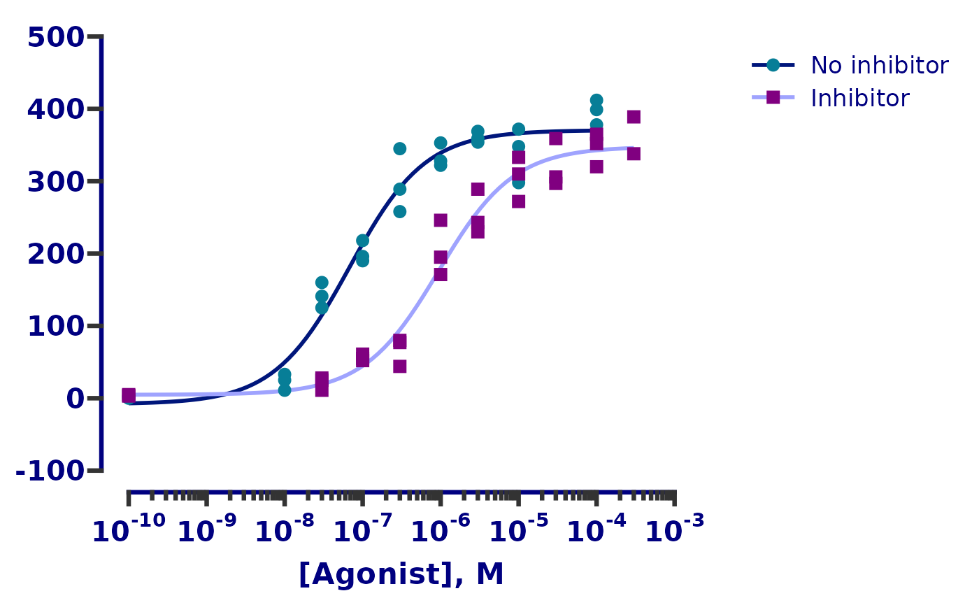
dose_resp <- y ~ min + ((max - min) / (1 + exp(hill_coefficient * (ec50 - x))))

ggplot(df, aes(x = log.agonist, y = response)) +
  geom_smooth(
    aes(colour = treatment),
    method = "nls", formula = dose_resp, se = FALSE,
    method.args = list(start = list(min = 1.67, max = 397, ec50 = -7, hill_coefficient = 1))
  ) +
  scale_colour_manual(labels = c("No inhibitor", "Inhibitor"),
                      values = c("#00167B", "#9FA3FE")) +
  ggnewscale::new_scale_colour() +
  geom_point(aes(colour = treatment, shape = treatment), size = 3) +
  scale_colour_prism(palette = "winter_bright",
                     labels = c("No inhibitor", "Inhibitor")) +
  scale_shape_prism(labels = c("No inhibitor", "Inhibitor")) +
  theme_prism(palette = "winter_bright", base_size = 16) +
  scale_y_continuous(limits = c(-100, 500),
                     breaks = seq(-100, 500, 100),
                     guide = "prism_offset") +
  scale_x_continuous(
    limits = c(-10, -3),
    breaks = -10:-3,
    guide = "prism_offset_minor",
    minor_breaks = log10(rep(1:9, 7)*(10^rep(-10:-4, each = 9))),
    labels = function(lab) {
      do.call(
        expression,
        lapply(paste(lab), function(x) bquote(bold("10"^.(x))))
      )
    }
  ) +
  theme(axis.title.y = element_blank(),
        legend.title = element_blank(),
        legend.position.inside = c(0.05, 0.95),
        legend.justification = c(0.05, 0.95)) +
  labs(x = "[Agonist], M")
#> Warning: The S3 guide system was deprecated in ggplot2 3.5.0.
#> ℹ It has been replaced by a ggproto system that can be extended.
#> This warning is displayed once every 8 hours.
#> Call `lifecycle::last_lifecycle_warnings()` to see where this warning was
#> generated.