Mixed Models

library(drcHelper)
source("../knitr-setup.R")

Variance Components

We first explore how variance components structure affect the dose-response analysis using the Intraclass Correlation Coefficient (ICC) patterns.

The ICC represents the proportion of total variance attributable to between-tank differences:

\[ \mbox{ICC} = \sigma^2_{between}/(\sigma^2_{between} + \sigma^2_{within}) \]

Example 1

# Let's simulate a single dataset with your existing function and examine its properties
set.seed(123)

# Simulate dose-response data with specific variance components
sim_data <- simulate_dose_response(
  n_doses = 5,
  dose_range = c(0, 20),
  m_tanks = 4,
  k_individuals = 10,
  var_tank = 6,     # Between-tank variance
  var_individual = 2,  # Within-tank (individual) variance
  include_individuals = TRUE,
  response_function = function(dose) {
    # Simple linear dose-response with threshold at dose 10
    ifelse(dose > 10, 5 + 2 * (dose - 10), 5)
  }
)

# Calculate theoretical ICC
theoretical_icc <- 6 / (6 + 2)  # var_tank / (var_tank + var_individual)
cat("Theoretical ICC:", theoretical_icc, "\n")
#> Theoretical ICC: 0.75

# Examine the data structure
head(sim_data)
#>   Dose Tank Individual Response
#> 1    0    1          1 2.116990
#> 2    0    1          3 3.318858
#> 3    0    4          1 2.985193
#> 4    0    4          3 3.405375
#> 5    0    3          2 7.934101
#> 6    0    2          1 2.787365
str(sim_data)
#> 'data.frame':    200 obs. of  4 variables:
#>  $ Dose      : num  0 0 0 0 0 0 0 0 0 0 ...
#>  $ Tank      : int  1 1 4 4 3 2 2 1 1 4 ...
#>  $ Individual: int  1 3 1 3 2 1 3 2 4 2 ...
#>  $ Response  : num  2.12 3.32 2.99 3.41 7.93 ...

# Visualize the data to see the hierarchical structure
library(ggplot2)

# Plot individual data points with tank means
ggplot(sim_data, aes(x = factor(Dose), y = Response, color = factor(Tank))) +
  geom_jitter(width = 0.2, alpha = 0.5) +
  stat_summary(fun = mean, geom = "point", size = 3) +
  stat_summary(fun = mean, geom = "line", aes(group = factor(Tank))) +
  labs(title = "Dose-Response Data with Hierarchical Structure",
       x = "Dose", y = "Response",
       color = "Tank") +
  theme_minimal()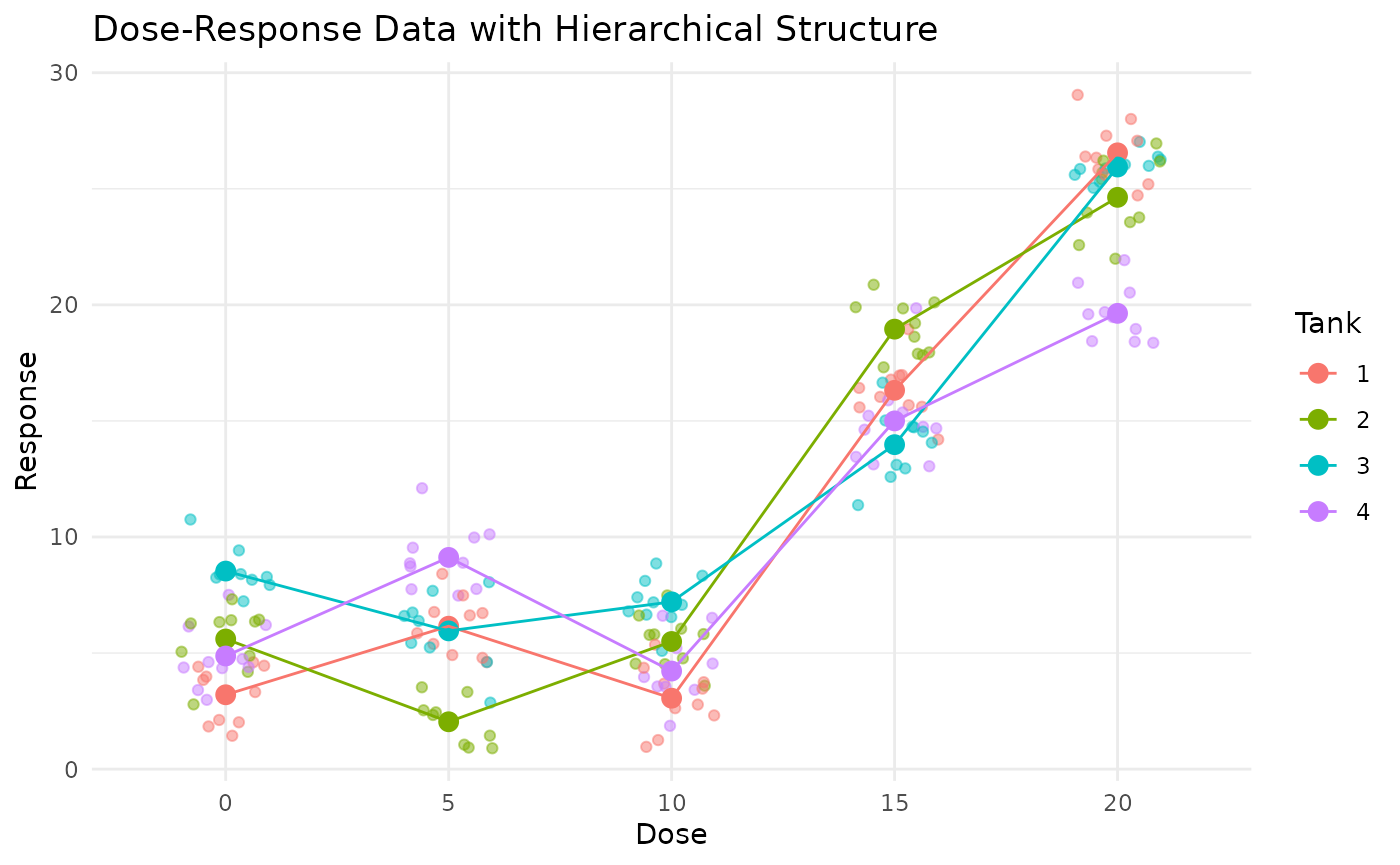

A plot generated from an R code chunk.


# Calculate observed ICC using a mixed model
library(lme4)
mixed_model <- lmer(Response ~ factor(Dose) + (1|Tank), data = sim_data)
summary(mixed_model)
#> Linear mixed model fit by REML ['lmerMod']
#> Formula: Response ~ factor(Dose) + (1 | Tank)
#>    Data: sim_data
#> 
#> REML criterion at convergence: 927.7
#> 
#> Scaled residuals: 
#>      Min       1Q   Median       3Q      Max 
#> -2.22011 -0.64124  0.04355  0.67388  2.79017 
#> 
#> Random effects:
#>  Groups   Name        Variance Std.Dev.
#>  Tank     (Intercept) 0.424    0.6511  
#>  Residual             6.060    2.4617  
#> Number of obs: 200, groups:  Tank, 4
#> 
#> Fixed effects:
#>                Estimate Std. Error t value
#> (Intercept)      5.5526     0.5074  10.942
#> factor(Dose)5    0.2649     0.5505   0.481
#> factor(Dose)10  -0.5574     0.5505  -1.013
#> factor(Dose)15  10.5100     0.5505  19.093
#> factor(Dose)20  18.6356     0.5505  33.855
#> 
#> Correlation of Fixed Effects:
#>             (Intr) fc(D)5 f(D)10 f(D)15
#> factor(Ds)5 -0.542                     
#> factr(Ds)10 -0.542  0.500              
#> factr(Ds)15 -0.542  0.500  0.500       
#> factr(Ds)20 -0.542  0.500  0.500  0.500

# Extract variance components
vc <- VarCorr(mixed_model)
tank_var <- as.numeric(vc$Tank)
residual_var <- attr(vc, "sc")^2
observed_icc <- tank_var / (tank_var + residual_var)
cat("Observed ICC:", observed_icc, "\n")
#> Observed ICC: 0.06538746

# Aggregate data to tank level
tank_data <- aggregate(Response ~ Dose + Tank, data = sim_data, FUN = mean)
head(tank_data)
#>   Dose Tank  Response
#> 1    0    1  3.202260
#> 2    5    1  6.156191
#> 3   10    1  3.054297
#> 4   15    1 16.318684
#> 5   20    1 26.548488
#> 6    0    2  5.604946

# Compare individual-level model with tank-level model
# Individual level (mixed model)
ind_model <- lmer(Response ~ factor(Dose) + (1|Tank), data = sim_data)

# Tank level (regular linear model)
tank_model <- lm(Response ~ factor(Dose), data = tank_data)

# Compare model summaries
summary(ind_model)
#> Linear mixed model fit by REML ['lmerMod']
#> Formula: Response ~ factor(Dose) + (1 | Tank)
#>    Data: sim_data
#> 
#> REML criterion at convergence: 927.7
#> 
#> Scaled residuals: 
#>      Min       1Q   Median       3Q      Max 
#> -2.22011 -0.64124  0.04355  0.67388  2.79017 
#> 
#> Random effects:
#>  Groups   Name        Variance Std.Dev.
#>  Tank     (Intercept) 0.424    0.6511  
#>  Residual             6.060    2.4617  
#> Number of obs: 200, groups:  Tank, 4
#> 
#> Fixed effects:
#>                Estimate Std. Error t value
#> (Intercept)      5.5526     0.5074  10.942
#> factor(Dose)5    0.2649     0.5505   0.481
#> factor(Dose)10  -0.5574     0.5505  -1.013
#> factor(Dose)15  10.5100     0.5505  19.093
#> factor(Dose)20  18.6356     0.5505  33.855
#> 
#> Correlation of Fixed Effects:
#>             (Intr) fc(D)5 f(D)10 f(D)15
#> factor(Ds)5 -0.542                     
#> factr(Ds)10 -0.542  0.500              
#> factr(Ds)15 -0.542  0.500  0.500       
#> factr(Ds)20 -0.542  0.500  0.500  0.500
summary(tank_model)
#> 
#> Call:
#> lm(formula = Response ~ factor(Dose), data = tank_data)
#> 
#> Residuals:
#>     Min      1Q  Median      3Q     Max 
#> -4.5543 -1.2816  0.1967  1.8654  3.3025 
#> 
#> Coefficients:
#>                Estimate Std. Error t value Pr(>|t|)    
#> (Intercept)      5.5526     1.2460   4.456 0.000462 ***
#> factor(Dose)5    0.2649     1.7621   0.150 0.882520    
#> factor(Dose)10  -0.5574     1.7621  -0.316 0.756118    
#> factor(Dose)15  10.5100     1.7621   5.964 2.59e-05 ***
#> factor(Dose)20  18.6356     1.7621  10.576 2.38e-08 ***
#> ---
#> Signif. codes:  0 '***' 0.001 '**' 0.01 '*' 0.05 '.' 0.1 ' ' 1
#> 
#> Residual standard error: 2.492 on 15 degrees of freedom
#> Multiple R-squared:  0.9261, Adjusted R-squared:  0.9063 
#> F-statistic: 46.96 on 4 and 15 DF,  p-value: 2.613e-08

# Extract and compare fixed effects
ind_fixed <- fixef(ind_model)
tank_fixed <- coef(tank_model)
cbind(ind_fixed,tank_fixed)
#>                 ind_fixed tank_fixed
#> (Intercept)     5.5525654  5.5525654
#> factor(Dose)5   0.2648670  0.2648670
#> factor(Dose)10 -0.5573896 -0.5573896
#> factor(Dose)15 10.5099513 10.5099513
#> factor(Dose)20 18.6355902 18.6355902

Example 2

Simualate a dose-response with unequal variances across the dose range.

# Example with increasing variance by dose
increasing_var_tank <- c(1, 2, 4, 8, 50)
increasing_var_individual <- c(0.5, 1, 1.5, 2, 2.5)

# Simulate data with inhomogeneous variance
sim_data_inhomogeneous <- simulate_dose_response(
  n_doses = 5,
  dose_range = c(0, 20),
  m_tanks = 3,
  k_individuals = 10,
  var_tank = increasing_var_tank,
  var_individual = increasing_var_individual,
  include_individuals = TRUE
)

prelimPlot3(sim_data_inhomogeneous%>% group_by(Dose,Tank)%>%summarise(Response=mean(Response),.groups = "drop"))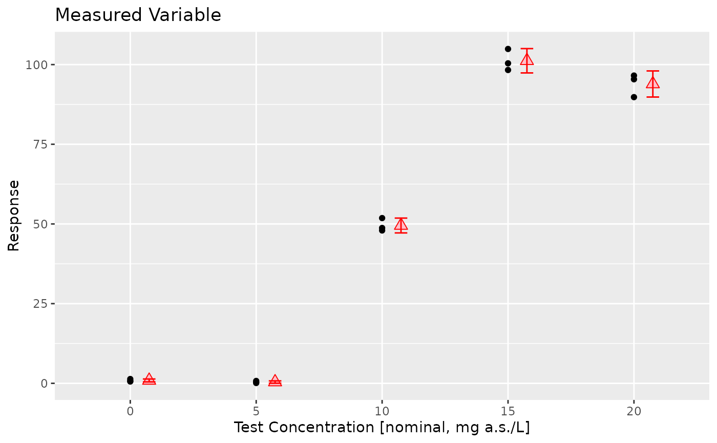

A plot generated from an R code chunk.

Expected Patterns in ICC and P-values Based on Variance Structures

Intraclass Correlation Coefficient (ICC) Patterns

The ICC represents the proportion of total variance attributable to between-tank differences:

\[ \mbox{ICC} = \sigma^2_{between}/(\sigma^2_{between} + \sigma^2_{within}) \]

Where: - \(\sigma^2_{between}\) is the between-tank variance (var_tank) - \(\sigma^2_{within}\) is the within-tank variance (var_individual)

Expected ICC Patterns:

High between-tank variance, low within-tank variance:
- ICC approaches 1.0
- Indicates strong tank effects where individuals within the same tank are highly similar
- Example: var_tank = 10, var_individual = 1 \(\rightarrow\) ICC \(\approx\) 0.91
Low between-tank variance, high within-tank variance:
- ICC approaches 0
- Indicates weak tank effects where individuals within the same tank vary substantially
- Example: var_tank = 1, var_individual = 10 \(\rightarrow\) ICC \(\approx\) 0.09
Equal between-tank and within-tank variance:
- ICC = 0.5
- Balanced contribution of tank and individual effects
- Example: var_tank = 4, var_individual = 4 \(\rightarrow\) ICC = 0.5

P-value Patterns in Relation to Variance Structure

Individual-Level Mixed Model vs. Tank-Level Aggregated Model:

High ICC Scenarios (strong tank effects):
- Tank-level model: Will perform nearly as well as the individual-level model
- Individual-level model: Gains little additional power from individual observations
- P-value comparison: Both models will produce similar p-values
- Efficiency: Tank-level analysis is more efficient computationally with minimal loss of statistical power
Low ICC Scenarios (weak tank effects):
- Tank-level model: Loses substantial information by aggregating highly variable individuals
- Individual-level model: Gains significant power from modeling individual observations
- P-value comparison: Individual-level model will typically produce lower p-values (higher power)
- Efficiency: Individual-level analysis is worth the computational cost due to increased power
Moderate ICC Scenarios:
- Trade-off zone: Balance between computational efficiency and statistical power
- P-value comparison: Individual-level model generally produces lower p-values, but the advantage diminishes as ICC increases

Effect of Variance Components on P-values:

Increasing between-tank variance (var_tank):
- Increases overall variability in the data
- Decreases statistical power for detecting dose effects
- Increases p-values in both models
- Makes tank-level aggregation more reasonable (higher ICC)
Increasing within-tank variance (var_individual):
- Increases variability at the individual level
- Decreases ICC
- Makes individual-level modeling more advantageous
- Tank-level model p-values will increase more dramatically than individual-level model p-values
Interaction with dose effect size:
- For small effect sizes: Variance structure has a more pronounced impact on p-values
- For large effect sizes: Both models may detect significant effects despite variance structure differences

Practical Implications

When to use tank-level analysis:
- High ICC scenarios (ICC > 0.7)
- When computational efficiency is a concern
- When the experimental design focuses on tank-level responses
When to use individual-level analysis:
- Low to moderate ICC scenarios (ICC < 0.7)
- When maximum statistical power is required
- When individual-level covariates are important
Variance heterogeneity across dose levels:
- If variance increases with dose, individual-level models with appropriate variance structures become more important
- Tank-level models may be less robust to variance heterogeneity

By systematically exploring these patterns through simulation, we can develop guidelines for choosing the appropriate analysis approach based on the specific variance structure in dose-response studies.

Why Sample Size Requirements Changes?

References

A cookbook in development

Development Notes

For multiple comparison using multcomp, there are several ways to code it in functions:

using do.call

 # Create a list for the mcp call
  mcp_list <- list("Dunnett")
  names(mcp_list) <- dose_var

  # Set control level if not the first level
  if (control_level != levels(data[[dose_var]])[1]) {
    control_idx <- which(levels(data[[dose_var]]) == as.character(control_level))
    mcp_list$base <- control_idx
  }
  
  dunnett_result <- multcomp::glht(model, linfct = do.call(multcomp::mcp, mcp_list))

using ``

# Create the mcp call as a string and then evaluate it
  mcp_call_str <- paste0("mcp(", dose_var, " = 'Dunnett')")
  if (control_level != levels(data[[dose_var]])[1]) {
    mcp_call_str <- paste0("mcp(", dose_var, " = 'Dunnett', base = ", control_idx, ")")
  }
  
  # Create the glht call as a string and then evaluate it
  glht_call_str <- paste0("glht(model, linfct = ", mcp_call_str, ")")
  # Evaluate the call, not sure if we need to add , envir = eval_env to the eval function.
  dunnett_result <- try(eval(parse(text = glht_call_str)), silent = TRUE)

Define the contrast matrix K, see drcHelper::dunnet_test for examples.