This file is to reproduce some drda results. drda is another R package for fitting dose-response curves, which includes additional Gompertz function. It was originally designed to fit nonlinear growth curves, using Newton’s with a trust-region method, which potentially is better in terms of optimization.
library(drcHelper)
#> Loading required package: drc
#> Loading required package: MASS
#> Loading required package: drcData
#>
#> 'drc' has been loaded.
#> Please cite R and 'drc' if used for a publication,
#> for references type 'citation()' and 'citation('drc')'.
#>
#> Attaching package: 'drc'
#> The following objects are masked from 'package:stats':
#>
#>     gaussian, getInitial
## remotes::install_github("albertopessia/drda")
library(drda)
Data
?voropm2

head(voropm2)
#>   response dose log_dose weight
#> 1   1.1263 1.00     0.00   0.87
#> 2   1.0329 1.00     0.00   1.04
#> 3   1.1139 1.00     0.00   0.94
#> 4   1.1146 1.93     0.66   0.96
#> 5   1.0664 1.93     0.66   0.91
#> 6   1.0163 1.93     0.66   0.93
Default Fitting
# by default `drda` uses a 4-parameter logistic function for model fitting

# common R API for fitting models
fit <- drda(response ~ log_dose, data = voropm2)

# get a general overview of the results
summary(fit)
#>
#> Call: drda(formula = response ~ log_dose, data = voropm2)
#>
#> Pearson Residuals:
#>      Min        1Q    Median        3Q       Max
#> -1.88121  -0.72514   0.06395   0.47905   2.17210
#>
#> Parameters:
#>                   Estimate Std. Error Lower .95 Upper .95
#> Maximum            1.04147    0.01022   1.02144     1.061
#> Height            -1.05659    0.02059  -1.09694    -1.016
#> Growth rate        3.07405    0.31744   2.45187     3.696
#> Midpoint at        6.53555    0.03593   6.46512     6.606
#> Residual std err.  0.05069    0.00574   0.03944     0.062
#>
#> Residual standard error on 41 degrees of freedom
#>
#> Log-likelihood: 72.432
#> AIC: -134.86
#> BIC: -125.83
#>
#> Optimization algorithm converged in 285 iterations

# get parameter estimates by using generic functions...
coef(fit)
#>     alpha     delta       eta       phi
#>  1.041465 -1.056586  3.074053  6.535548
sigma(fit)
#> [1] 0.05069196

# ... or accessing the variables directly
fit$coefficients
#>     alpha     delta       eta       phi
#>  1.041465 -1.056586  3.074053  6.535548
fit$sigma
#> [1] 0.05069196

# compare the estimated model against a flat horizontal line, or the full
# 5-parameter logistic model, using AIC, BIC, and the Likelihood Ratio Test
# (LRT)
#
# note that the LRT is testing the null hypothesis of a flat horizontal line
# being as a good fit as the chosen model, therefore we expect the test to be
# significant
#
# if the test is not significant, a horizontal line is probably a better model
anova(fit)
#> Analysis of Deviance Table
#>
#> Model 1: a
#> Model 2: a + d / (1 + exp(-e * (x - p))) (Fit)
#> Model 3: a + d / (1 + n * exp(-e * (x - p)))^(1 / n) (Full)
#>
#> Model 3 is the best model according to the Akaike Information Criterion.
#>
#>         Resid. Df Resid. Dev Df      AIC     BIC Deviance    LRT  Pr(>Chi)
#> Model 1        44     9.0879  1   59.717   63.33
#> Model 2        41     0.1054  4 -134.864 -125.83  -8.9825 200.58 < 2.2e-16 ***
#> Model 3        40     0.0773  5 -146.774 -135.93  -0.0280  13.91 0.0001917 ***
#> ---
#> Signif. codes:  0 '***' 0.001 '**' 0.01 '*' 0.05 '.' 0.1 ' ' 1
Other models
# use the `mean_function` argument to select a different model
fit_l2 <- drda(response ~ log_dose, data = voropm2, mean_function = "logistic2")
fit_l4 <- drda(response ~ log_dose, data = voropm2, mean_function = "logistic4")
fit_l5 <- drda(response ~ log_dose, data = voropm2, mean_function = "logistic5")
fit_gz <- drda(response ~ log_dose, data = voropm2, mean_function = "gompertz")

# which model should be chosen?
anova(fit_l2, fit_l4, fit_l5, fit_gz)
#> Analysis of Deviance Table
#>
#> Model 1: a
#> Model 2: 1 - 1 / (1 + exp(-e * (x - p)))
#> Model 3: a + d * exp(-exp(-e * (x - p)))
#> Model 4: a + d / (1 + exp(-e * (x - p)))
#> Model 5: a + d / (1 + n * exp(-e * (x - p)))^(1 / n) (Full)
#>
#> Model 5 is the best model according to the Akaike Information Criterion.
#>
#>         Resid. Df Resid. Dev Df      AIC     BIC Deviance     LRT  Pr(>Chi)
#> Model 1        44     9.0879      59.717   63.33
#> Model 2        43     0.1493  1 -123.180 -117.76  -8.9386 184.897 < 2.2e-16 ***
#> Model 3        41     0.1438  2 -120.873 -111.84  -0.0055   1.692 0.4291117
#> Model 4        41     0.1054  0 -134.864 -125.83  -0.0384  13.991
#> Model 5        40     0.0773  1 -146.774 -135.93  -0.0280  13.910 0.0001917 ***
#> ---
#> Signif. codes:  0 '***' 0.001 '**' 0.01 '*' 0.05 '.' 0.1 ' ' 1

# 5-parameter logistic function provides the best fit (AIC and BIC are minimum)
Weighted fit
# it is possible to give each observation its own weight
fit_weighted <- drda(response ~ log_dose, data = voropm2, weights = weight)

# all the commands shown so far are available for a weighted fit as well
Constrained optimization
# it is possible to fix parameter values by setting the `lower_bound` and
# `upper_bound` appropriately
#
# unconstrained parameters have a lower bound of `-Inf` and an upper bound of
# `Inf`
#
# Important: be careful when deciding the constraints, because the optimization
#            problem might become very difficult to solve within a reasonable
#            number of iterations.
#
# In this particular example we are:
#   - fixing the alpha parameter to 1
#   - fixing the delta parameter to -1
#   - constraining the growth rate to be between 1 and 5
#   - not constraining the `phi` parameter, i.e. the `log(EC50)`
lb <- c(1, -1, 1, -Inf)
ub <- c(1, -1, 5,  Inf)

fit <- drda(
  response ~ log_dose, data = voropm2, lower_bound = lb, upper_bound = ub,
  max_iter = 260
)

summary(fit)
#>
#> Call: drda(formula = response ~ log_dose, data = voropm2, lower_bound = lb,
#>     upper_bound = ub, max_iter = 260)
#>
#> Pearson Residuals:
#>      Min        1Q    Median        3Q       Max
#> -1.76281  -0.14933   0.08862   0.81283   2.56716
#>
#> Parameters:
#>                   Estimate Std. Error Lower .95 Upper .95
#> Maximum            1.00000         NA        NA        NA
#> Height            -1.00000         NA        NA        NA
#> Growth rate        3.58631   0.448736   2.70680     4.466
#> Midpoint at        6.57056   0.035336   6.50130     6.640
#> Residual std err.  0.05893   0.006432   0.04632     0.072
#>
#> Residual standard error on 43 degrees of freedom
#>
#> Log-likelihood: 64.584
#> AIC: -123.17
#> BIC: -117.75
#>
#> Optimization algorithm DID NOT converge in 260 iterations

# if the algorithm does not converge, we can try to increase the maximum number
# of iterations or provide our own starting point
fit <- drda(
  response ~ log_dose, data = voropm2, lower_bound = lb, upper_bound = ub,
  start = c(1, -1, 2.6, 5), max_iter = 10000
)

summary(fit)
#>
#> Call: drda(formula = response ~ log_dose, data = voropm2, lower_bound = lb,
#>     upper_bound = ub, start = c(1, -1, 2.6, 5), max_iter = 10000)
#>
#> Pearson Residuals:
#>      Min        1Q    Median        3Q       Max
#> -1.78762  -0.14935   0.08877   0.81294   2.56740
#>
#> Parameters:
#>                   Estimate Std. Error Lower .95 Upper .95
#> Maximum            1.00000         NA        NA        NA
#> Height            -1.00000         NA        NA        NA
#> Growth rate        3.62475   0.464908   2.71355     4.536
#> Midpoint at        6.56865   0.035267   6.49953     6.638
#> Residual std err.  0.05892   0.006429   0.04632     0.072
#>
#> Residual standard error on 43 degrees of freedom
#>
#> Log-likelihood: 64.59
#> AIC: -123.18
#> BIC: -117.76
#>
#> Optimization algorithm converged in 284 iterations
Plotting
fit_l5 <- drda(response ~ log_dose, data = voropm2, mean_function = "logistic5")

# plot the data used for fitting, the maximum likelihood curve, and
# *approximate* confidence intervals for the curve
plot(fit_l5)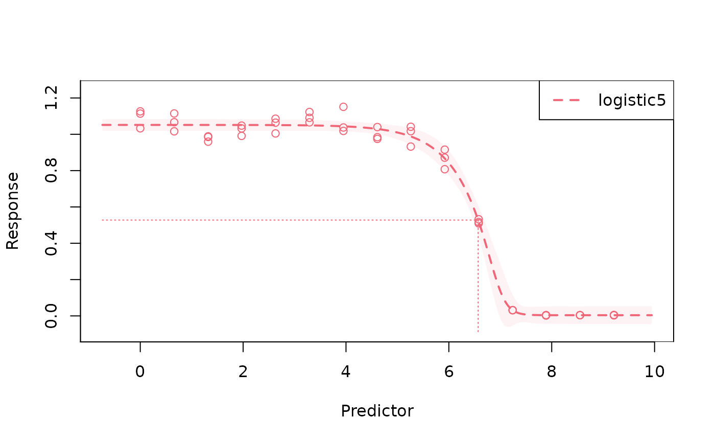
# combine all curves in the same plot
fit_l2 <- drda(response ~ log_dose, data = voropm2, mean_function = "logistic2")
fit_l4 <- drda(response ~ log_dose, data = voropm2, mean_function = "logistic4")
plot(fit_l2, fit_l4, fit_l5)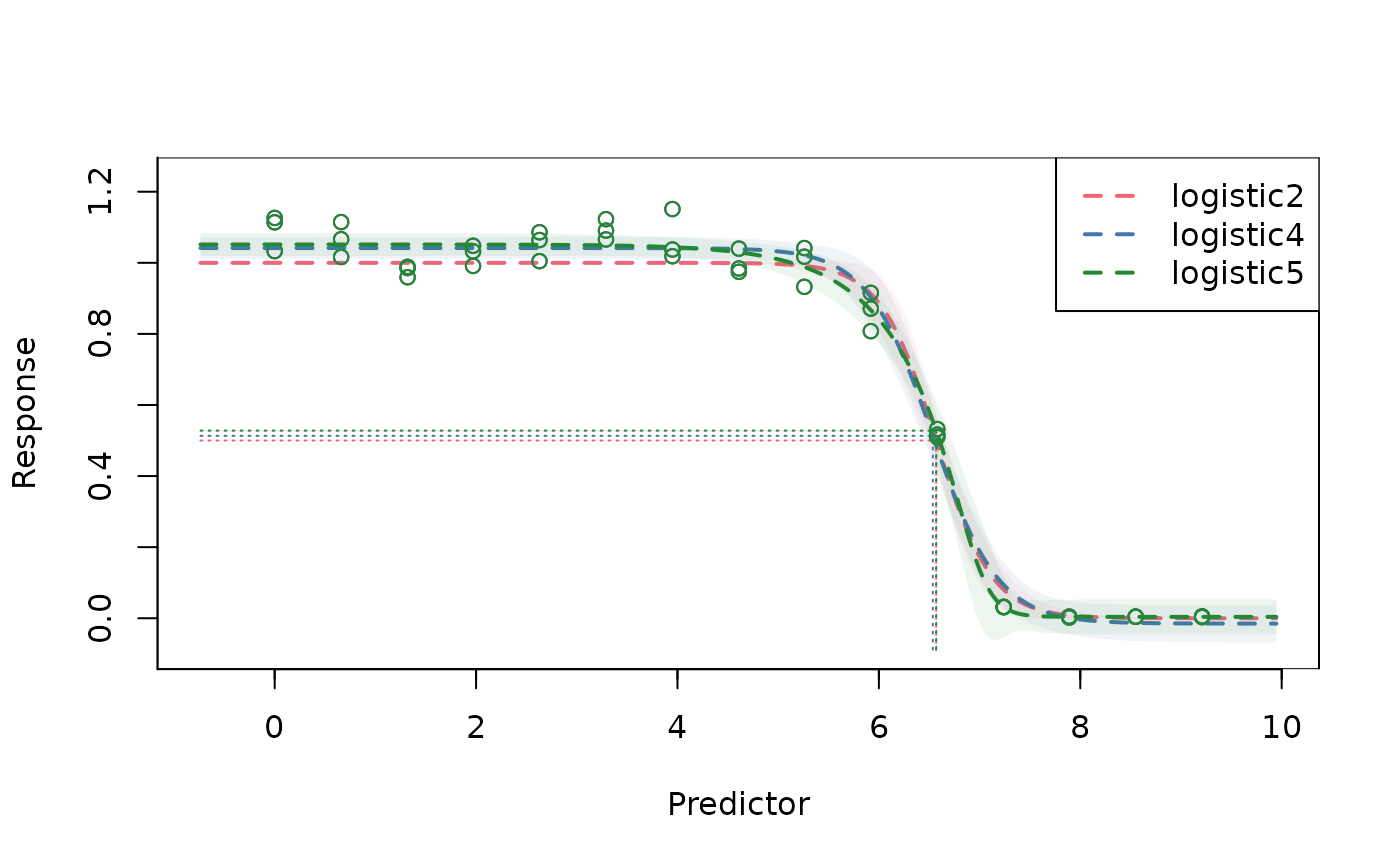
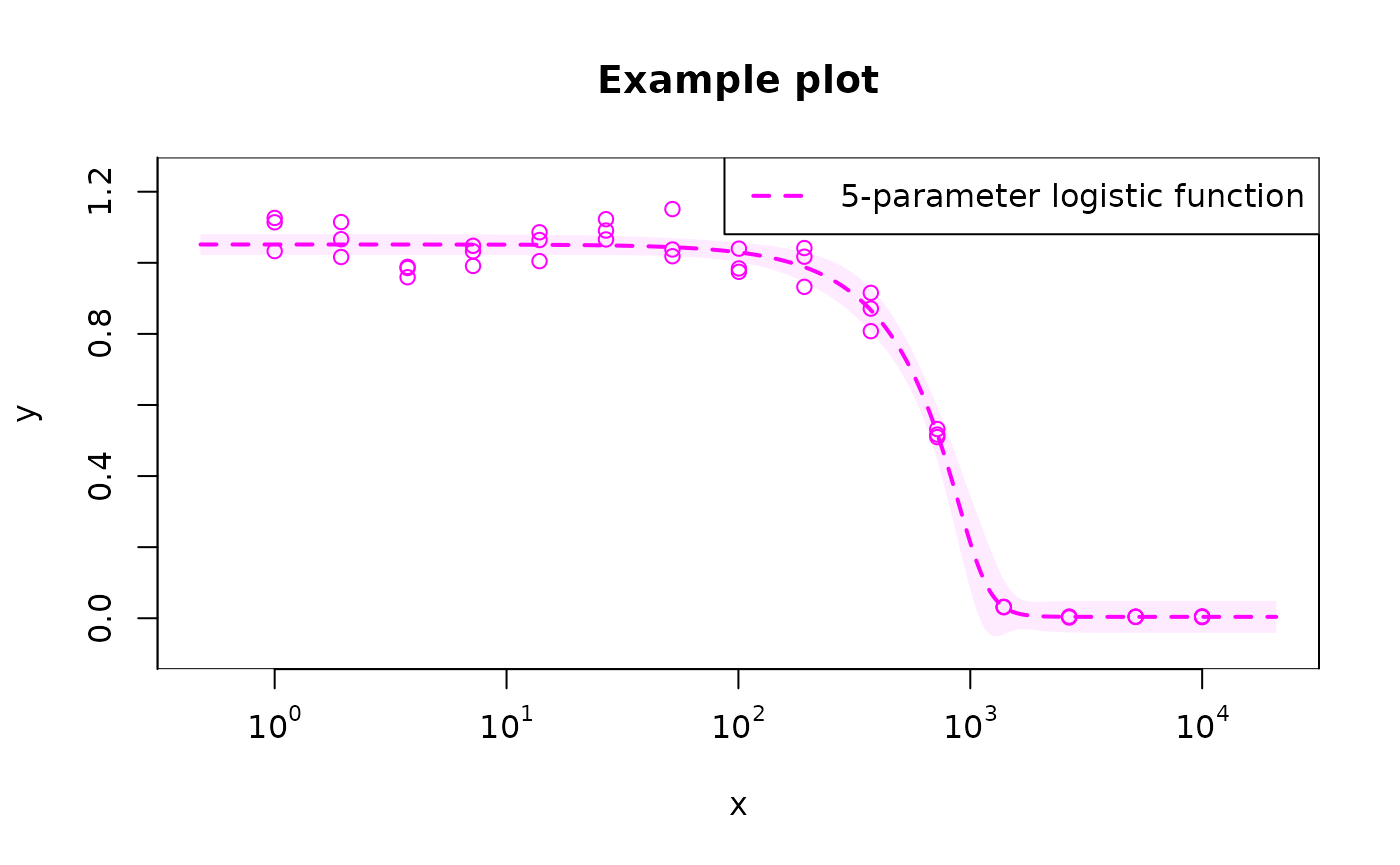
# modify default plotting options
# use `legend_show = FALSE` to remove the legend altogether
plot(
  fit_l5, base = "10", col = "magenta", xlab = "x", ylab = "y", level = 0.9,
  midpoint = FALSE, main = "Example plot", legend_location = "topright",
  legend = "5-parameter logistic function"
)
References
Malyutina A, Tang J, Pessia A (2023). drda: An R package for dose-response data analysis using logistic functions. Journal of Statistical Software, 106(4), 1-26. doi:10.18637/jss.v106.i04