Data Overview
sum1 <- oecd201 %>% group_by(Time,Treatment) %>% summarise(Yield_mean=mean(Yield),Yield_sd=sd(Yield),GrowthRate_mean=mean(GrowthRate),GrowthRate_sd=sd(GrowthRate))
sum0 <- sum1%>%filter(Treatment=="Control")%>%rename(Yield0=Yield_mean,GrowthRate0=GrowthRate_mean)%>%dplyr::select(c(Time,Yield0,GrowthRate0))
# sum0
sumtab <- left_join(sum1%>%filter(Time>0),sum0) %>% mutate(Yield_Inhibition=(Yield0-Yield_mean)/Yield0*100,GrowthRate_Inhibition=(GrowthRate0-GrowthRate_mean)/GrowthRate0*100) %>% dplyr::select(c(Time,Treatment,Yield_mean,Yield_sd,Yield_Inhibition,GrowthRate_mean,GrowthRate_sd,GrowthRate_Inhibition))
sumtab%>%dplyr::select(c(Yield_mean,Yield_sd,Yield_Inhibition))%>%filter(Time==72)%>%knitr::kable(.,digits = 2,caption="<center><strong>Yield Summary at Time 72h<strong><center>",escape = FALSE)%>% kableExtra::kable_styling(bootstrap_options = "striped")##%>%kableExtra::kable_classic_2()
Yield Summary at Time 72h
|
Time
|
Yield_mean
|
Yield_sd
|
Yield_Inhibition
|
|
72
|
56.26
|
3.97
|
0.00
|
|
72
|
51.57
|
2.79
|
8.33
|
|
72
|
52.11
|
4.72
|
7.38
|
|
72
|
19.22
|
0.49
|
65.84
|
|
72
|
2.47
|
0.13
|
95.61
|
|
72
|
0.45
|
0.62
|
99.20
|
|
72
|
0.64
|
1.07
|
98.86
|
sumtab%>%dplyr::select(c(GrowthRate_mean,GrowthRate_sd,GrowthRate_Inhibition))%>%filter(Time==72)%>%knitr::kable(.,digits = 2,caption="<center><strong>Growth Rate Summary at Time 72h<strong><center>",escape = FALSE)##%>%kableExtra::kable_classic()
Table:
Growth Rate Summary at Time 72h
| 72 |
1.35 |
0.02 |
0.00 |
| 72 |
1.32 |
0.02 |
2.09 |
| 72 |
1.32 |
0.03 |
1.89 |
| 72 |
1.00 |
0.01 |
25.69 |
| 72 |
0.41 |
0.01 |
69.25 |
| 72 |
0.09 |
0.18 |
93.04 |
| 72 |
0.09 |
0.28 |
93.16 |
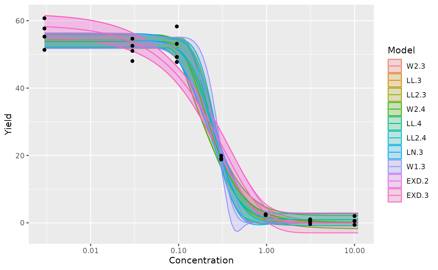
Model Fitting and Comparison For Yield
datTn<- subset(oecd201,Time==72)

mod <- drm(Yield~Concentration,data=datTn,fct=LL.3())
fctList <- list(LL2.3(),W2.3(),W1.3(),EXD.3(),EXD.2(),LN.3(),W2.4(),LL.4(),LL2.4())
plot(mod,type="all")

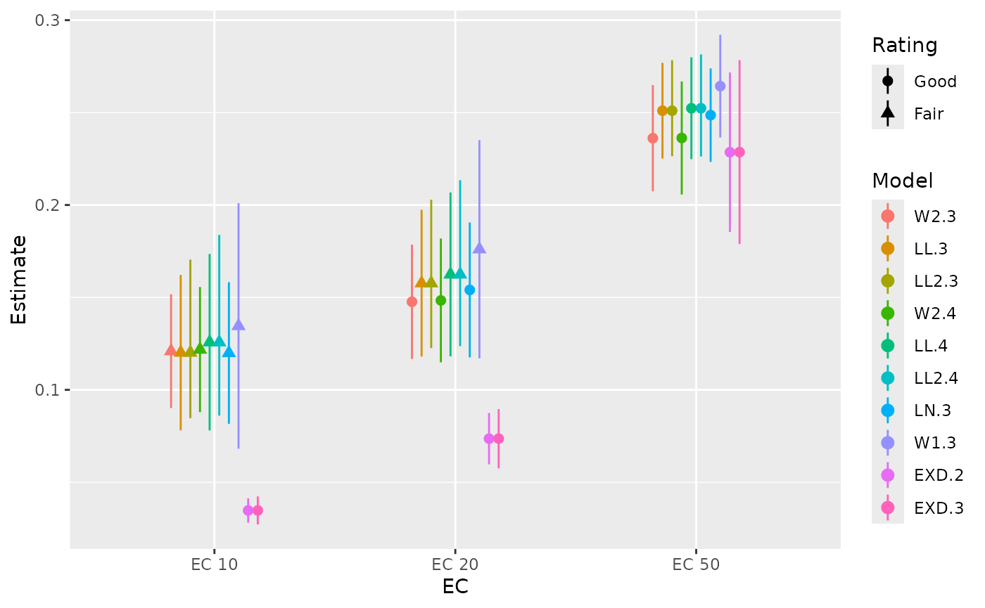
res <- mselect.plus(mod,fctList = fctList )
modList <- res$modList
edResTab <- mselect.ED(modList = modList,respLev = c(10,20,50),trend=datTn$Trend_Yield[1])
plot_edList(edResTab)
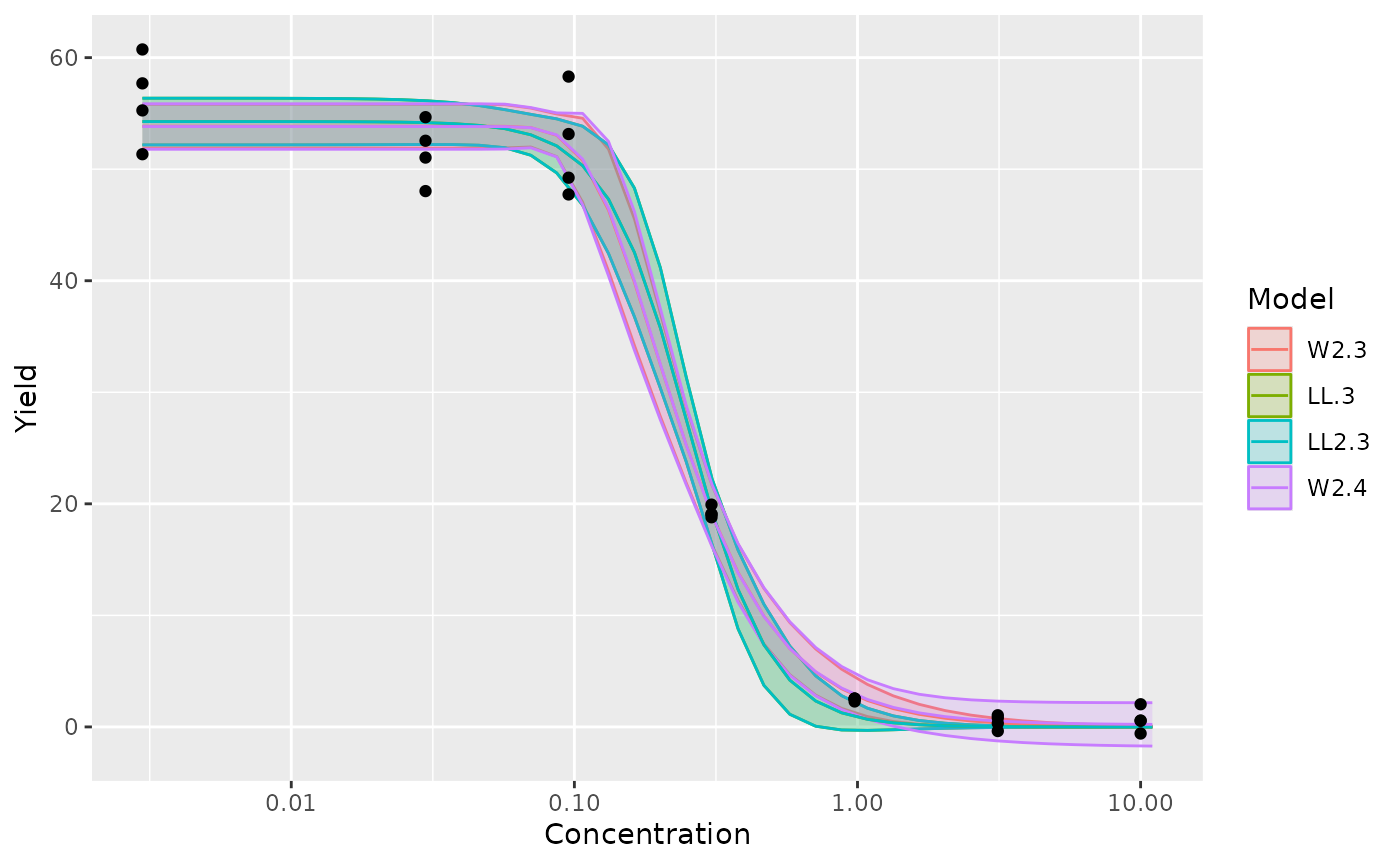
resComp <- drcCompare(modRes = res,trend="Decrease")
knitr::kable(edResTab,caption = "14 day TSL Yield",digits = 3)
14 day TSL Yield
| W2.3 |
0.121 |
0.015 |
0.090 |
0.152 |
0.509 |
Fair |
EC 10 |
| W2.3 |
0.148 |
0.015 |
0.117 |
0.179 |
0.419 |
Good |
EC 20 |
| W2.3 |
0.236 |
0.014 |
0.207 |
0.265 |
0.243 |
Good |
EC 50 |
| LL.3 |
0.120 |
0.020 |
0.078 |
0.162 |
0.700 |
Fair |
EC 10 |
| LL.3 |
0.158 |
0.019 |
0.118 |
0.197 |
0.504 |
Fair |
EC 20 |
| LL.3 |
0.251 |
0.013 |
0.225 |
0.277 |
0.206 |
Good |
EC 50 |
| LL2.3 |
0.120 |
NA |
0.085 |
0.170 |
0.714 |
Fair |
EC 10 |
| LL2.3 |
0.158 |
NA |
0.123 |
0.203 |
0.509 |
Fair |
EC 20 |
| LL2.3 |
0.251 |
NA |
0.226 |
0.278 |
0.207 |
Good |
EC 50 |
| W2.4 |
0.122 |
0.016 |
0.088 |
0.156 |
0.556 |
Fair |
EC 10 |
| W2.4 |
0.148 |
0.016 |
0.115 |
0.182 |
0.451 |
Good |
EC 20 |
| W2.4 |
0.236 |
0.015 |
0.206 |
0.267 |
0.259 |
Good |
EC 50 |
| LL.4 |
0.126 |
0.023 |
0.078 |
0.173 |
0.759 |
Fair |
EC 10 |
| LL.4 |
0.162 |
0.021 |
0.118 |
0.207 |
0.546 |
Fair |
EC 20 |
| LL.4 |
0.252 |
0.013 |
0.225 |
0.280 |
0.218 |
Good |
EC 50 |
| LL2.4 |
0.126 |
NA |
0.086 |
0.184 |
0.777 |
Fair |
EC 10 |
| LL2.4 |
0.162 |
NA |
0.124 |
0.213 |
0.552 |
Fair |
EC 20 |
| LL2.4 |
0.252 |
NA |
0.226 |
0.281 |
0.219 |
Good |
EC 50 |
| LN.3 |
0.120 |
0.019 |
0.082 |
0.158 |
0.639 |
Fair |
EC 10 |
| LN.3 |
0.154 |
0.018 |
0.118 |
0.191 |
0.474 |
Good |
EC 20 |
| LN.3 |
0.249 |
0.012 |
0.223 |
0.274 |
0.203 |
Good |
EC 50 |
| W1.3 |
0.135 |
0.032 |
0.068 |
0.201 |
0.987 |
Fair |
EC 10 |
| W1.3 |
0.176 |
0.029 |
0.117 |
0.235 |
0.671 |
Fair |
EC 20 |
| W1.3 |
0.264 |
0.013 |
0.237 |
0.292 |
0.210 |
Good |
EC 50 |
| EXD.2 |
0.035 |
0.003 |
0.028 |
0.041 |
0.378 |
Good |
EC 10 |
| EXD.2 |
0.074 |
0.007 |
0.060 |
0.087 |
0.378 |
Good |
EC 20 |
| EXD.2 |
0.229 |
0.021 |
0.185 |
0.272 |
0.378 |
Good |
EC 50 |
| EXD.3 |
0.035 |
0.004 |
0.027 |
0.042 |
0.435 |
Good |
EC 10 |
| EXD.3 |
0.074 |
0.008 |
0.058 |
0.090 |
0.435 |
Good |
EC 20 |
| EXD.3 |
0.229 |
0.024 |
0.179 |
0.278 |
0.435 |
Good |
EC 50 |
knitr::kable(resComp,caption = "14 day TSL Yield, Model Comparison",digits = 3)
14 day TSL Yield, Model Comparison
| W2.3 |
-66.456 |
140.912 |
0.188 |
7.556 |
Medium |
Medium |
0 |
| LL.3 |
-67.245 |
142.489 |
0.117 |
7.994 |
Medium |
Medium |
0 |
| LL2.3 |
-67.245 |
142.489 |
0.117 |
7.994 |
High |
Medium |
0 |
| W2.4 |
-66.433 |
142.866 |
0.113 |
7.858 |
Medium |
Medium |
0 |
| LL.4 |
-66.584 |
143.169 |
0.102 |
7.943 |
Medium |
Medium |
0 |
| LL2.4 |
-66.584 |
143.169 |
0.102 |
7.943 |
Medium |
Medium |
0 |
| LN.3 |
-67.745 |
143.490 |
0.086 |
8.284 |
Medium |
Medium |
0 |
| W1.3 |
-68.086 |
144.173 |
0.069 |
8.489 |
Medium |
Medium |
0 |
| EXD.2 |
-80.603 |
167.207 |
0.000 |
19.958 |
High |
Shallow |
0 |
| EXD.3 |
-80.603 |
169.207 |
0.000 |
20.756 |
High |
Shallow |
0 |
p <-plot.modList(modList[c(1)],scale="logx",npts=80)+theme(legend.position = "none")+ggtitle("14 day Total Shoot Length, \n3-parameter type II Weibull Model Fit")
addECxCI(p=p,object=modList[[1]],EDres=NULL,trend="Decrease",endpoint="EC", respLev=c(10,20,50),
                     textAjust.x=0.01,textAjust.y=1,useObsCtr=FALSE,d0=NULL,textsize = 4,lineheight = 1,xmin=0.012)+ylab("Total Shoot Length [cm]") + xlab("Concentration [µg a.s./L]")
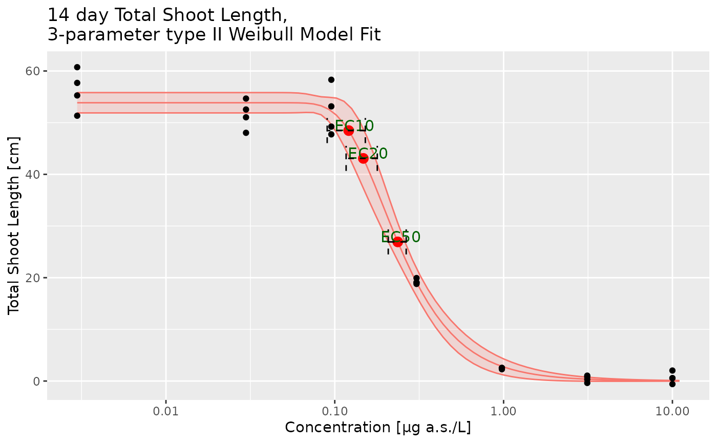
resED <- t(edResTab[1:3, c(2,4,5,6)])
colnames(resED) <- paste("EC", c(10,20,50))
knitr::kable(resED,caption = "Total Shoot Length Growth Yield at 14 day",digits = 3)
Total Shoot Length Growth Yield at 14 day
| Estimate |
0.121 |
0.148 |
0.236 |
| Lower |
0.090 |
0.117 |
0.207 |
| Upper |
0.152 |
0.179 |
0.265 |
| NW |
0.509 |
0.419 |
0.243 |
| EC 5 |
0.1044 |
0.01464 |
0.0743 |
0.1346 |
| EC 10 |
0.1209 |
0.01494 |
0.09017 |
0.1517 |
| EC 20 |
0.1477 |
0.01501 |
0.1167 |
0.1786 |
| EC 50 |
0.2361 |
0.01395 |
0.2074 |
0.2649 |
| b:(Intercept) |
-1.794 |
0.2203 |
-8.144 |
1.696e-08 |
| d:(Intercept) |
53.85 |
0.9535 |
56.48 |
3.42e-28 |
| e:(Intercept) |
0.1925 |
0.01447 |
13.3 |
7.664e-13 |