In a nutshell, an equivalence test is conducted if you want to provide strong support for the absence of a meaningful effect. A often used procedure is two onse-sided tests. It means you need to be able to reject two null hypothesis to conclude equivalence with some confidence. Interestingly, we will be still using the same confidence intervals as in difference testing, but need to use the 90% CI and need this CI to be completely included in the predefined range of “no meaningful differences”.
It should be noted that studies designed under the difference testing framework would not be suitable for direct switch to equivalence test, the power requirement is just different. Even though we are using a narrower CI (from 95% to 90%), we need the entire CI fit inside the predefined bounds, on the other hand, a difference test just require the point of zero falling into the CI. Therefore, we would need a much tighter CI so that the full length fits within.
Introduction
Equivalence testing is a statistical testing approach used to determine whether two treatments or interventions produce effects that are practically the same within a predefined margin of difference. This method is particularly useful in fields like pharmaceuticals, where demonstrating that a new drug is not worse than an existing one by more than a specified margin is crucial.
Equivalence testing is closely related to difference testing. While the latter focuses on identifying whether a difference exists by controlling the false positive error, the former aims to show that any difference is within a predefined acceptable range, by controlling the false negative error in the difference testing scenario.
he design and interpretation of equivalence tests can be more complex than traditional difference tests, requiring careful consideration of the equivalence margin, which could be so called biologically relevant effect size.
The null and alternative hypotheses in equivalence tests are
\[ H_0: | \mu_1 - \mu_0 | > \Delta \] \[ H_1: | \mu_1 - \mu_0 | \leq \Delta \] where \(\mu_1\) and \(\mu_0\) are the means of the two treatments, and \(\Delta\) is the equivalence margin.
There are also non-inferiority or non-superiority cases, where the nulls are \(\mu_1 - \mu_0 <= - \Delta\) or \(\mu_1 - \mu_0 > \Delta\)
Sometimes the tests can be formulated on standardized differences or means. Depending on how you frame the problem, the multiplicative model for ratios-to-control comparisons could be used. Related approach is available
The \(\alpha\) level in equivalence testing is the probability of making a Type I error, which occurs when the null hypothesis is incorrectly rejected. This means concluding that the treatments are equivalent when they are not.
The \(\beta\) in difference testing is the probability of making a Type II error, which occurs when the null hypothesis is not rejected when it should be. This means failing to detect a difference (concluding equivalence) when one actually exists.
In equivalence testing, a low alpha level is crucial to ensure that the conclusion of equivalence is reliable. Conversely, in difference testing, a low beta level is important to ensure that a true difference is detected.
On the other hand, the \(\alpha\) level in difference testing is playing similarly a complementary role to the \(\beta\) in equivalence testing.
The Confusion
If thinking from the confidence interval (CI) direction, the equivalence testing uses the 90% CI for confidence level of 95% (\(\alpha = 0.05\)). We illustrate it here.
The switch from 95% to 90% confidence intervals in equivalence testing is actually a simple mathematical approach to maintain an overall 5% Type I error rate (95% confidence) in our conclusion about equivalence.
In equivalence testing, we need to show that BOTH the upper and lower bounds of our confidence interval fall within our predefined zone of indifference.
When we use a 90% confidence interval, we have:
- 5% error probability in the upper tail
- 5% error probability in the lower tail
- (Because 100% - 90% = 10%, split equally between two tails)
- For equivalence to be concluded, we need both bounds to fall within our zone of indifference. The probability of this happening by chance (if the treatments aren’t truly equivalent) is approximately 5% because:
- We multiply the probability of success for each bound (0.95 × 0.95 ≈ 0.90)
- This gives us 95% confidence in our overall conclusion about equivalence
So while we’re using a 90% confidence interval as our tool, the end result gives us 95% confidence in our conclusion about equivalence. This approach effectively controls the overall Type I error rate at the traditional 5% level, maintaining the statistical rigor we expect in hypothesis testing.
This is why equivalence testing protocols specifically call for 90% confidence intervals - it’s not a reduction in our confidence standards, but rather a mathematical adjustment to achieve the desired 95% confidence in our final conclusion about equivalence.
Impacts of changing from difference to equivalence testing
- Equivalence testing often requires larger sample sizes to achieve sufficient power, which can be resource-intensive.
- The design and interpretation of equivalence tests can be more complex than traditional difference tests, requiring careful consideration of the “equivalence margin”.
Hypothetical Examples
I will simulate a dose response
library(drcHelper)
n_doses <- 5
dose_range <- c(0,20)
## Define a threshold dose response
threshold_idx  <-  3 ## kind of global
doses <- seq(dose_range[1], dose_range[2], length.out = n_doses)
response_fn <- function(dose, max_effect) {
  base_response <- 100
  result <- rep(base_response, length(dose))
  threshold_dose <- doses[threshold_idx]
  high_doses <- dose >= threshold_dose
  if (any(high_doses)) {
    max_high_dose <- max(doses)
    relative_position <- (dose[high_doses] - threshold_dose) / (max_high_dose - threshold_dose)
    result[high_doses] <- base_response - relative_position * max_effect
  }
  return(result)
}


max_effect <- 5
sim_data <- simulate_dose_response(
  n_doses = 5,
  dose_range = c(0,20),
  m_tanks = 10,
  var_tank = 3,  # Pass the dose-specific variances, note here it should be a vector instead of a singe number.
  include_individuals = FALSE,  # Tank-level data only
  response_function = function(dose) response_fn(dose, max_effect)
)
theme_set(theme_bw())
prelimPlot3(sim_data)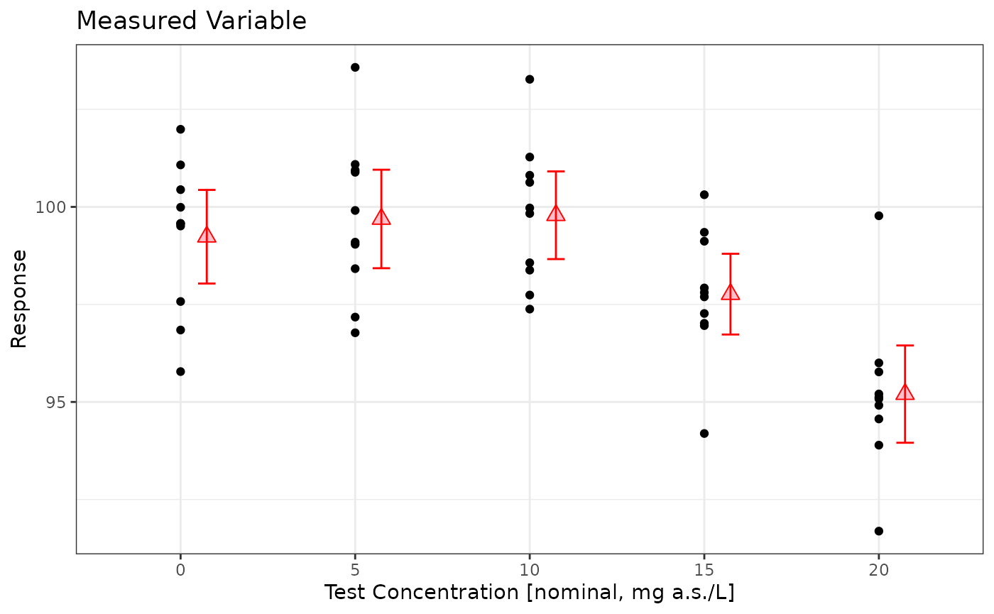
mod <- lm(Response~Dose, data=sim_data %>% dplyr::mutate(Dose=factor(Dose)))
summary(mod)
#>
#> Call:
#> lm(formula = Response ~ Dose, data = sim_data %>% dplyr::mutate(Dose = factor(Dose)))
#>
#> Residuals:
#>     Min      1Q  Median      3Q     Max
#> -3.5719 -1.1151  0.0437  1.1540  4.5715
#>
#> Coefficients:
#>             Estimate Std. Error t value Pr(>|t|)
#> (Intercept)  99.2355     0.6003 165.302  < 2e-16 ***
#> Dose5         0.4550     0.8490   0.536   0.5947
#> Dose10        0.5505     0.8490   0.648   0.5200
#> Dose15       -1.4720     0.8490  -1.734   0.0898 .
#> Dose20       -4.0345     0.8490  -4.752 2.09e-05 ***
#> ---
#> Signif. codes:  0 '***' 0.001 '**' 0.01 '*' 0.05 '.' 0.1 ' ' 1
#>
#> Residual standard error: 1.898 on 45 degrees of freedom
#> Multiple R-squared:  0.4789, Adjusted R-squared:  0.4325
#> F-statistic: 10.34 on 4 and 45 DF,  p-value: 5.039e-06
library(multcomp)
summary(glht(mod,linfct = mcp(Dose="Dunnett")))
#>
#>   Simultaneous Tests for General Linear Hypotheses
#>
#> Multiple Comparisons of Means: Dunnett Contrasts
#>
#>
#> Fit: lm(formula = Response ~ Dose, data = sim_data %>% dplyr::mutate(Dose = factor(Dose)))
#>
#> Linear Hypotheses:
#>             Estimate Std. Error t value Pr(>|t|)
#> 5 - 0 == 0    0.4550     0.8490   0.536    0.954
#> 10 - 0 == 0   0.5505     0.8490   0.648    0.915
#> 15 - 0 == 0  -1.4720     0.8490  -1.734    0.258
#> 20 - 0 == 0  -4.0345     0.8490  -4.752   <0.001 ***
#> ---
#> Signif. codes:  0 '***' 0.001 '**' 0.01 '*' 0.05 '.' 0.1 ' ' 1
#> (Adjusted p values reported -- single-step method)

summary(glht(mod,linfct = mcp(Dose="Dunnett"), alternative="greater", rhs=-10 ))
#>
#>   Simultaneous Tests for General Linear Hypotheses
#>
#> Multiple Comparisons of Means: Dunnett Contrasts
#>
#>
#> Fit: lm(formula = Response ~ Dose, data = sim_data %>% dplyr::mutate(Dose = factor(Dose)))
#>
#> Linear Hypotheses:
#>               Estimate Std. Error t value Pr(>t)
#> 5 - 0 <= -10    0.4550     0.8490  12.315 <1e-08 ***
#> 10 - 0 <= -10   0.5505     0.8490  12.427 <1e-08 ***
#> 15 - 0 <= -10  -1.4720     0.8490  10.045 <1e-08 ***
#> 20 - 0 <= -10  -4.0345     0.8490   7.026 <1e-08 ***
#> ---
#> Signif. codes:  0 '***' 0.001 '**' 0.01 '*' 0.05 '.' 0.1 ' ' 1
#> (Adjusted p values reported -- single-step method)
summary(glht(mod,linfct = mcp(Dose="Dunnett"), alternative="less", rhs= 10 ))
#>
#>   Simultaneous Tests for General Linear Hypotheses
#>
#> Multiple Comparisons of Means: Dunnett Contrasts
#>
#>
#> Fit: lm(formula = Response ~ Dose, data = sim_data %>% dplyr::mutate(Dose = factor(Dose)))
#>
#> Linear Hypotheses:
#>              Estimate Std. Error t value Pr(<t)
#> 5 - 0 >= 10    0.4550     0.8490  -11.24 <1e-10 ***
#> 10 - 0 >= 10   0.5505     0.8490  -11.13 <1e-10 ***
#> 15 - 0 >= 10  -1.4720     0.8490  -13.51 <1e-10 ***
#> 20 - 0 >= 10  -4.0345     0.8490  -16.53 <1e-10 ***
#> ---
#> Signif. codes:  0 '***' 0.001 '**' 0.01 '*' 0.05 '.' 0.1 ' ' 1
#> (Adjusted p values reported -- single-step method)
confint(glht(mod,linfct = mcp(Dose="Dunnett")),level=0.9)
#>
#>   Simultaneous Confidence Intervals
#>
#> Multiple Comparisons of Means: Dunnett Contrasts
#>
#>
#> Fit: lm(formula = Response ~ Dose, data = sim_data %>% dplyr::mutate(Dose = factor(Dose)))
#>
#> Quantile = 2.2218
#> 90% family-wise confidence level
#>
#>
#> Linear Hypotheses:
#>             Estimate lwr     upr
#> 5 - 0 == 0   0.4550  -1.4314  2.3413
#> 10 - 0 == 0  0.5505  -1.3359  2.4368
#> 15 - 0 == 0 -1.4720  -3.3583  0.4144
#> 20 - 0 == 0 -4.0345  -5.9209 -2.1482
max_effect <- 10
sim_data <- simulate_dose_response(
  n_doses = 5,
  dose_range = c(0,20),
  m_tanks = 10,
  var_tank = 3,  # Pass the dose-specific variances, note here it should be a vector instead of a singe number.
  include_individuals = FALSE,  # Tank-level data only
  response_function = function(dose) response_fn(dose, max_effect)
)
theme_set(theme_bw())
prelimPlot3(sim_data)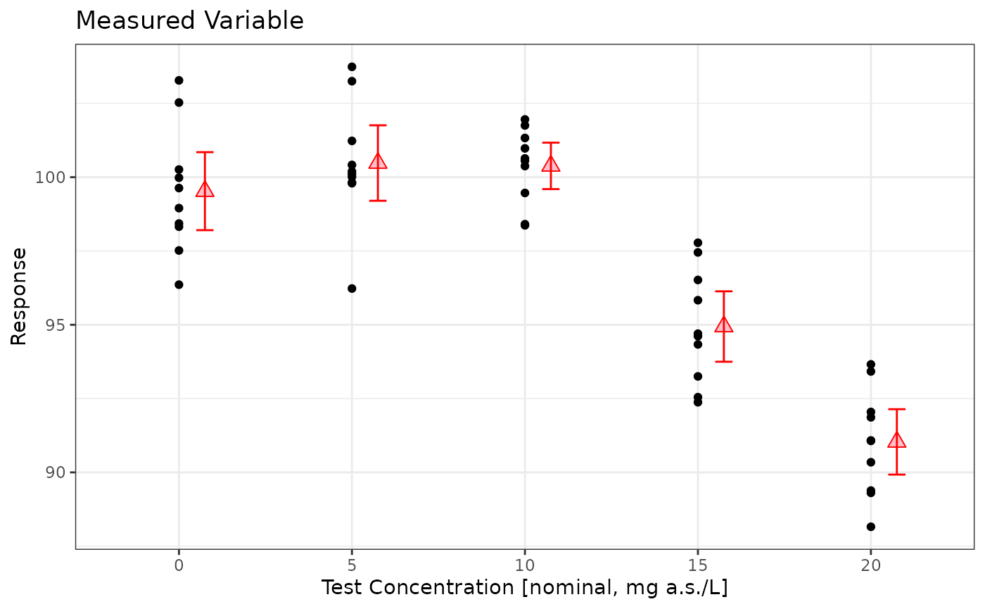
mod <- lm(Response~Dose, data=sim_data %>% dplyr::mutate(Dose=factor(Dose)))
summary(mod)
#>
#> Call:
#> lm(formula = Response ~ Dose, data = sim_data %>% dplyr::mutate(Dose = factor(Dose)))
#>
#> Residuals:
#>     Min      1Q  Median      3Q     Max
#> -4.2513 -1.0514 -0.0348  0.9322  3.7530
#>
#> Coefficients:
#>             Estimate Std. Error t value Pr(>|t|)
#> (Intercept)  99.5264     0.5884 169.154  < 2e-16 ***
#> Dose5         0.9532     0.8321   1.146    0.258
#> Dose10        0.8564     0.8321   1.029    0.309
#> Dose15       -4.5858     0.8321  -5.511 1.65e-06 ***
#> Dose20       -8.4936     0.8321 -10.208 2.72e-13 ***
#> ---
#> Signif. codes:  0 '***' 0.001 '**' 0.01 '*' 0.05 '.' 0.1 ' ' 1
#>
#> Residual standard error: 1.861 on 45 degrees of freedom
#> Multiple R-squared:  0.8167, Adjusted R-squared:  0.8004
#> F-statistic: 50.13 on 4 and 45 DF,  p-value: 5.108e-16
library(multcomp)
summary(glht(mod,linfct = mcp(Dose="Dunnett")))
#>
#>   Simultaneous Tests for General Linear Hypotheses
#>
#> Multiple Comparisons of Means: Dunnett Contrasts
#>
#>
#> Fit: lm(formula = Response ~ Dose, data = sim_data %>% dplyr::mutate(Dose = factor(Dose)))
#>
#> Linear Hypotheses:
#>             Estimate Std. Error t value Pr(>|t|)
#> 5 - 0 == 0    0.9532     0.8321   1.146    0.611
#> 10 - 0 == 0   0.8564     0.8321   1.029    0.693
#> 15 - 0 == 0  -4.5858     0.8321  -5.511   <1e-04 ***
#> 20 - 0 == 0  -8.4936     0.8321 -10.208   <1e-04 ***
#> ---
#> Signif. codes:  0 '***' 0.001 '**' 0.01 '*' 0.05 '.' 0.1 ' ' 1
#> (Adjusted p values reported -- single-step method)

summary(glht(mod,linfct = mcp(Dose="Dunnett"), alternative="greater", rhs=-10 ))
#>
#>   Simultaneous Tests for General Linear Hypotheses
#>
#> Multiple Comparisons of Means: Dunnett Contrasts
#>
#>
#> Fit: lm(formula = Response ~ Dose, data = sim_data %>% dplyr::mutate(Dose = factor(Dose)))
#>
#> Linear Hypotheses:
#>               Estimate Std. Error t value Pr(>t)
#> 5 - 0 <= -10    0.9532     0.8321  13.163 <0.001 ***
#> 10 - 0 <= -10   0.8564     0.8321  13.047 <0.001 ***
#> 15 - 0 <= -10  -4.5858     0.8321   6.507 <0.001 ***
#> 20 - 0 <= -10  -8.4936     0.8321   1.810  0.113
#> ---
#> Signif. codes:  0 '***' 0.001 '**' 0.01 '*' 0.05 '.' 0.1 ' ' 1
#> (Adjusted p values reported -- single-step method)
summary(glht(mod,linfct = mcp(Dose="Dunnett"), alternative="less", rhs= 10 ))
#>
#>   Simultaneous Tests for General Linear Hypotheses
#>
#> Multiple Comparisons of Means: Dunnett Contrasts
#>
#>
#> Fit: lm(formula = Response ~ Dose, data = sim_data %>% dplyr::mutate(Dose = factor(Dose)))
#>
#> Linear Hypotheses:
#>              Estimate Std. Error t value Pr(<t)
#> 5 - 0 >= 10    0.9532     0.8321  -10.87 <1e-10 ***
#> 10 - 0 >= 10   0.8564     0.8321  -10.99 <1e-10 ***
#> 15 - 0 >= 10  -4.5858     0.8321  -17.53 <1e-10 ***
#> 20 - 0 >= 10  -8.4936     0.8321  -22.23 <1e-10 ***
#> ---
#> Signif. codes:  0 '***' 0.001 '**' 0.01 '*' 0.05 '.' 0.1 ' ' 1
#> (Adjusted p values reported -- single-step method)
confint(glht(mod,linfct = mcp(Dose="Dunnett")),level=0.9)
#>
#>   Simultaneous Confidence Intervals
#>
#> Multiple Comparisons of Means: Dunnett Contrasts
#>
#>
#> Fit: lm(formula = Response ~ Dose, data = sim_data %>% dplyr::mutate(Dose = factor(Dose)))
#>
#> Quantile = 2.2223
#> 90% family-wise confidence level
#>
#>
#> Linear Hypotheses:
#>             Estimate lwr      upr
#> 5 - 0 == 0    0.9532  -0.8960   2.8024
#> 10 - 0 == 0   0.8564  -0.9928   2.7056
#> 15 - 0 == 0  -4.5858  -6.4350  -2.7366
#> 20 - 0 == 0  -8.4936 -10.3428  -6.6444
max_effect <- 15
threshold_idx <- 1
 response_fn <- function(dose, max_effect) {
      base_response <- 100
      mid_dose <- mean(dose_range)
      return(base_response - max_effect * (1 - ((dose - mid_dose)/(mid_dose))^2)) ## Here I need a change.
 }
  response_fn <- function(dose, lower = 100, upper = 0, ED50 = 10, slope = 1) {
      lower + (upper - lower) / (1 + exp(-slope * (dose - ED50)))
  }
  set.seed(456)
sim_data <- simulate_dose_response(
  n_doses = 10,
  dose_range = c(0,20),
  m_tanks = 5,
  var_tank = 20,  # Pass the dose-specific variances, note here it should be a vector instead of a singe number.
  include_individuals = FALSE,  # Tank-level data only
  response_function = function(dose) response_fn(dose, max_effect)
)
theme_set(theme_bw())

sim_data <-sim_data %>% dplyr::mutate(Dose = round(Dose, 2))
prelimPlot3(sim_data)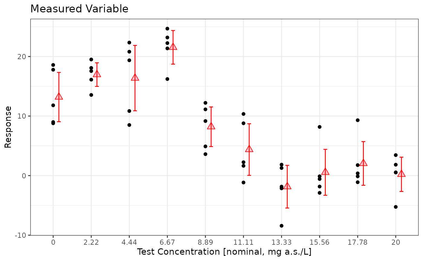
mod <- lm(Response~Dose, data=sim_data %>% dplyr::filter(Dose <=15) %>%
            dplyr::mutate(Dose=factor(Dose)))
summary(mod)
#>
#> Call:
#> lm(formula = Response ~ Dose, data = sim_data %>% dplyr::filter(Dose <=
#>     15) %>% dplyr::mutate(Dose = factor(Dose)))
#>
#> Residuals:
#>     Min      1Q  Median      3Q     Max
#> -7.8720 -3.3567  0.5979  3.1387  5.9788
#>
#> Coefficients:
#>             Estimate Std. Error t value Pr(>|t|)
#> (Intercept)   13.189      1.945   6.780 2.31e-07 ***
#> Dose2.22       3.771      2.751   1.371  0.18140
#> Dose4.44       3.182      2.751   1.157  0.25722
#> Dose6.67       8.351      2.751   3.036  0.00514 **
#> Dose8.89      -4.986      2.751  -1.812  0.08065 .
#> Dose11.11     -8.814      2.751  -3.204  0.00337 **
#> Dose13.33    -15.047      2.751  -5.469 7.70e-06 ***
#> ---
#> Signif. codes:  0 '***' 0.001 '**' 0.01 '*' 0.05 '.' 0.1 ' ' 1
#>
#> Residual standard error: 4.35 on 28 degrees of freedom
#> Multiple R-squared:  0.7893, Adjusted R-squared:  0.7441
#> F-statistic: 17.48 on 6 and 28 DF,  p-value: 2.64e-08
library(multcomp)


summary(glht(mod,linfct = mcp(Dose="Dunnett"), alternative="greater", rhs=-10 ))
#>
#>   Simultaneous Tests for General Linear Hypotheses
#>
#> Multiple Comparisons of Means: Dunnett Contrasts
#>
#>
#> Fit: lm(formula = Response ~ Dose, data = sim_data %>% dplyr::filter(Dose <=
#>     15) %>% dplyr::mutate(Dose = factor(Dose)))
#>
#> Linear Hypotheses:
#>                  Estimate Std. Error t value Pr(>t)
#> 2.22 - 0 <= -10     3.771      2.751   5.005 <0.001 ***
#> 4.44 - 0 <= -10     3.182      2.751   4.791 <0.001 ***
#> 6.67 - 0 <= -10     8.351      2.751   6.670 <0.001 ***
#> 8.89 - 0 <= -10    -4.986      2.751   1.822  0.149
#> 11.11 - 0 <= -10   -8.814      2.751   0.431  0.709
#> 13.33 - 0 <= -10  -15.047      2.751  -1.834  0.999
#> ---
#> Signif. codes:  0 '***' 0.001 '**' 0.01 '*' 0.05 '.' 0.1 ' ' 1
#> (Adjusted p values reported -- single-step method)
summary(glht(mod,linfct = mcp(Dose="Dunnett"), alternative="less", rhs= 10 ))
#>
#>   Simultaneous Tests for General Linear Hypotheses
#>
#> Multiple Comparisons of Means: Dunnett Contrasts
#>
#>
#> Fit: lm(formula = Response ~ Dose, data = sim_data %>% dplyr::filter(Dose <=
#>     15) %>% dplyr::mutate(Dose = factor(Dose)))
#>
#> Linear Hypotheses:
#>                 Estimate Std. Error t value Pr(<t)
#> 2.22 - 0 >= 10     3.771      2.751  -2.264 0.0667 .
#> 4.44 - 0 >= 10     3.182      2.751  -2.478 0.0431 *
#> 6.67 - 0 >= 10     8.351      2.751  -0.599 0.6369
#> 8.89 - 0 >= 10    -4.986      2.751  -5.447 <0.001 ***
#> 11.11 - 0 >= 10   -8.814      2.751  -6.839 <0.001 ***
#> 13.33 - 0 >= 10  -15.047      2.751  -9.104 <0.001 ***
#> ---
#> Signif. codes:  0 '***' 0.001 '**' 0.01 '*' 0.05 '.' 0.1 ' ' 1
#> (Adjusted p values reported -- single-step method)

summary(glht(mod,linfct = mcp(Dose="Dunnett")))
#>
#>   Simultaneous Tests for General Linear Hypotheses
#>
#> Multiple Comparisons of Means: Dunnett Contrasts
#>
#>
#> Fit: lm(formula = Response ~ Dose, data = sim_data %>% dplyr::filter(Dose <=
#>     15) %>% dplyr::mutate(Dose = factor(Dose)))
#>
#> Linear Hypotheses:
#>                Estimate Std. Error t value Pr(>|t|)
#> 2.22 - 0 == 0     3.771      2.751   1.371   0.5692
#> 4.44 - 0 == 0     3.182      2.751   1.157   0.7183
#> 6.67 - 0 == 0     8.351      2.751   3.036   0.0248 *
#> 8.89 - 0 == 0    -4.986      2.751  -1.812   0.3011
#> 11.11 - 0 == 0   -8.814      2.751  -3.204   0.0167 *
#> 13.33 - 0 == 0  -15.047      2.751  -5.469   <0.001 ***
#> ---
#> Signif. codes:  0 '***' 0.001 '**' 0.01 '*' 0.05 '.' 0.1 ' ' 1
#> (Adjusted p values reported -- single-step method)
confint(glht(mod,linfct = mcp(Dose="Dunnett")),level=0.9)
#>
#>   Simultaneous Confidence Intervals
#>
#> Multiple Comparisons of Means: Dunnett Contrasts
#>
#>
#> Fit: lm(formula = Response ~ Dose, data = sim_data %>% dplyr::filter(Dose <=
#>     15) %>% dplyr::mutate(Dose = factor(Dose)))
#>
#> Quantile = 2.4082
#> 90% family-wise confidence level
#>
#>
#> Linear Hypotheses:
#>                Estimate lwr      upr
#> 2.22 - 0 == 0    3.7705  -2.8548  10.3958
#> 4.44 - 0 == 0    3.1819  -3.4434   9.8072
#> 6.67 - 0 == 0    8.3512   1.7259  14.9765
#> 8.89 - 0 == 0   -4.9864 -11.6116   1.6389
#> 11.11 - 0 == 0  -8.8137 -15.4390  -2.1884
#> 13.33 - 0 == 0 -15.0467 -21.6720 -8.4214References
- Dilba, G., Bretz, F., Guiard, V., and Hothorn, L. A. (2004). Simultaneous confidence intervals for ratios with applications to the comparison of several treatments with a control. Methods of Information in Medicine 43, 465–469.
- Djira G, Hasler M, Gerhard D, Segbehoe L, Schaarschmidt F (2025). mratios: Ratios of Coefficients in the General Linear Model. R package version 1.4.4, https://CRAN.R-project.org/package=mratios.