Spearman-Karber Estimation with Modified Handling for Control Mortality

Estimates the LC50 (median lethal concentration) or ED50 (median effective dose) and its confidence interval using the Spearman-Karber method. This version includes robust handling for zero-dose (control) mortality and a Fieller-like approach for confidence interval estimation when control mortality is non-zero.

Usage

SpearmanKarber_modified(
  conc,
  dead,
  total,
  conf.level = 0.95,
  retData = TRUE,
  showOutput = FALSE,
  showPlot = FALSE
)

Arguments

conc: A numeric vector of doses or concentrations (must be >= 0 and in increasing order).
dead: A numeric vector of the number of organisms that died or responded at each conc level.
total: A numeric vector of the total number of organisms (population size) at each conc level. Can be a single value if all are the same.
conf.level: A single numeric value specifying the confidence level for the interval estimation (e.g., 0.95 for a 95% CI). Must be in (0, 1).
retData: A logical value. If TRUE, the results are returned in a list. If FALSE, invisible(NULL) is returned.
showOutput: A logical value. If TRUE, the input data table and estimation results (including log-scale values and CIs) are printed to the console.
showPlot: A logical value. If TRUE, a plot is generated showing the observed and Abbott-corrected mortalities/responses, the estimated LC50, and its confidence interval.

Value

A list containing the estimation results if retData is TRUE, otherwise invisible(NULL). The list includes:

log10LC50: Estimated log10 of the LC50.
varianceOfLog10LC50: Estimated variance of log10LC50.
StandardDeviationOfm: Estimated standard deviation of log10LC50.
confidenceIntervalLog10: CI for log10LC50 (vector of two values).
LC50: Estimated LC50 (10^log10LC50).
confidenceIntervalLC50: CI for LC50 (vector of two values).
conf.level: The confidence level used for the CIs.

Details

The function operates in two branches:

If control mortality (p0) is near zero, the standard Spearman-Karber method is used on the log-transformed doses, assuming the first observed response is 0%.
If p0 is non-zero, it estimates the background rate (c) by cumulative pooling, Abbott-corrects the proportions, prunes/pools low-dose groups, and uses a modified Spearman-Karber method on the scaled proportions. Confidence intervals are calculated using an approach inspired by Fieller's theorem to account for the background correction uncertainty.

All concentrations must be non-negative and in increasing order.

References

ART CARTER, WYETH-AYERST RESEARCH, CHAZY, NY (1994): Using the Spearman-Karber Method to Estimate the ED50. Proceedings of the Nineteenth Annual SAS Users Group International Conference, Dallas, Texas, April, pp. 10-13. http://www.sascommunity.org/sugi/SUGI94/Sugi-94-195%20Carter.pdf.

Author

Sarah Baumert, Harald Schulz, Zhenglei Gao

Examples

# Example 1: Zero control mortality (standard Spearman-Karber)
x1 <- c(0, 0.2, 0.3, 0.375, 0.625, 2)
n1 <- c(30, 30, 30, 30, 30, 30)
r1 <- c(0, 1, 3, 16, 24, 30)
SpearmanKarber_modified(x1, r1, n1, showOutput = TRUE)
#>  idx concentration total dead obs_prop abbott_prop abbott_count
#>    1         0.000    30    0 0.000000    0.000000            0
#>    2         0.200    30    1 0.033333    0.033333            1
#>    3         0.300    30    3 0.100000    0.100000            3
#>    4         0.375    30   16 0.533333    0.533333           16
#>    5         0.625    30   24 0.800000    0.800000           24
#>    6         2.000    30   30 1.000000    1.000000           30
#> log10(LC50) = -0.3468666 
#> estimated variance of log10(LC50) = 0.0009713409 
#> approx. half-width on log10-scale = 0.06108491 
#> 95% CI for log10(LC50) = [-0.40795150200696, -0.285781685210433]
#> estimated LC50 = 0.449918 
#> estimated 95% CI for LC50 = [0.390884543727692, 0.517867092299863]
#> $log10LC50
#> [1] -0.3468666
#> 
#> $varianceOfLog10LC50
#> [1] 0.0009713409
#> 
#> $StandardDeviationOfm
#> [1] 0.03116634
#> 
#> $confidenceIntervalLog10
#> [1] -0.4079515 -0.2857817
#> 
#> $LC50
#> [1] 0.449918
#> 
#> $confidenceIntervalLC50
#> [1] 0.3908845 0.5178671
#> 
#> $conf.level
#> [1] 0.95
#> 

# Example 2: Non-zero control mortality (modified method)
x2 <- c(0, 15.54, 20.47, 27.92, 35.98, 55.52)
n2 <- c(40, 40, 40, 40, 40, 40)
r2 <- c(3, 2, 6, 11, 18, 33)
results <- SpearmanKarber_modified(x2, r2, n2, retData = TRUE,
                                   showOutput = TRUE, showPlot = TRUE)

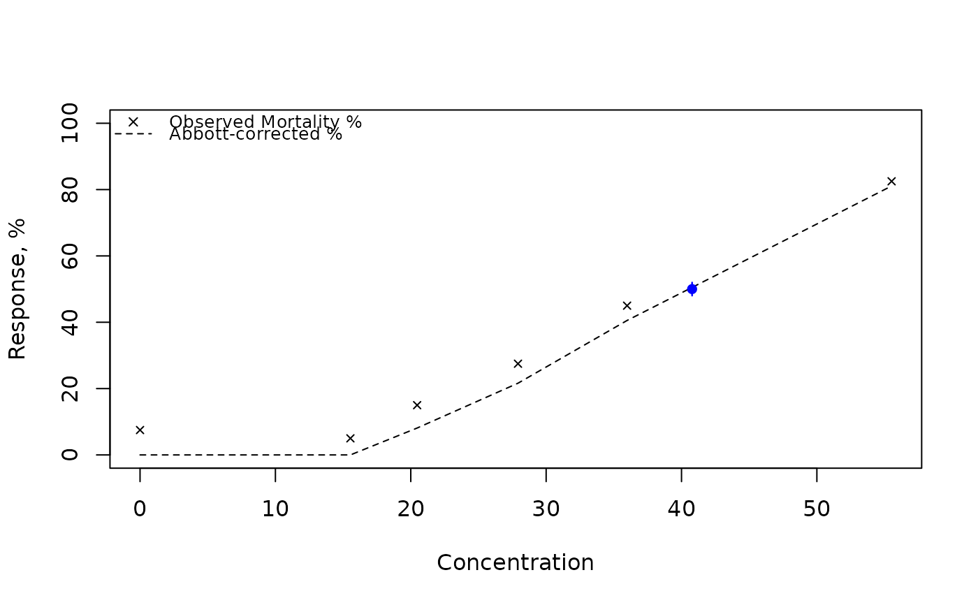#>  idx concentration total dead obs_prop abbott_prop abbott_count
#>    1          0.00    40    3    0.075    0.000000        0.000
#>    2         15.54    40    2    0.050    0.000000        0.000
#>    3         20.47    40    6    0.150    0.081081        3.243
#>    4         27.92    40   11    0.275    0.216216        8.649
#>    5         35.98    40   18    0.450    0.405405       16.216
#>    6         55.52    40   33    0.825    0.810811       32.432
#> log10(LC50) = 1.61046 
#> estimated variance of log10(LC50) = 0.0002126237 
#> approx. half-width on log10-scale = 0 
#> 95% CI for log10(LC50) = [1.61046032692499, 1.61046032692499]
#> estimated LC50 = 40.78123 
#> estimated 95% CI for LC50 = [40.781230615809, 40.781230615809]
print(results$LC50)
#> [1] 40.78123